
Risk, Odds, and Causality: A Practical Guide for Epidemiology and Healthcare AI
Published:
Risk, Odds, and Causality: A Practical Guide for Epidemiology and Healthcare AI
An illustrated primer on statistical associations, causal reasoning, and meaningful interpretation of health data.
Clinicians, epidemiologists, and healthcare practitioners seek to understand why disease occurs, which treatments work, and how best to care for patients. Computer scientists encounter the same questions when building disease-prediction systems, integrating medical images with electronic records, or studying population-health datasets. Yet a highly accurate disease predictor, a statistically significant odds ratio, and a credible causal effect estimate answer different questions. Understanding their differences starts with the language of exposures, outcomes, probabilities, and interventions.
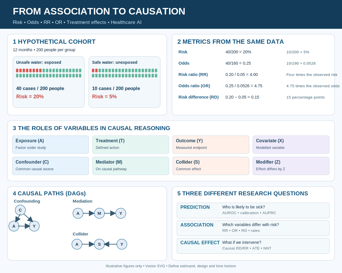
An overview of the illustrative example. Select the image to view it at full size.
1. One running example: water exposure and infection
Imagine an illustrative, rather than real, 12-month cohort study of 400 people initially free of gastrointestinal infection. Researchers observe 200 people who drink unsafe water and 200 people who drink safe water. By the end of follow-up, 40 in the unsafe-water group and 10 in the safe-water group develop infection.
| Group | Infection | No infection | Total |
|---|---|---|---|
| Exposed: unsafe water | 40 | 160 | 200 |
| Unexposed: safe water | 10 | 190 | 200 |
In standard notation, a=40, b=160, c=10 and d=190. This table summarises an association, not automatically a causal effect. People using unsafe water may differ in sanitation, living conditions, access to care, and other factors.
Why specify the time frame?
Risk is a probability during a specified interval, not a timeless attribute. “20% risk” is incomplete unless we know whether it means during hospitalisation, 30 days, 12 months, or a lifetime. Valid comparison also requires an appropriate population at risk, comparable outcome ascertainment, and suitable handling of loss to follow-up. If events can recur, defining the first event versus repeated episodes also changes the estimand.
2. Essential terminology before doing the calculations
Exposure
An exposure is the variable whose relationship to the outcome is being examined. It may be an environmental condition (unsafe water), behaviour (smoking), medication use, blood-pressure category, biomarker level, or imaging-derived phenotype. It is not necessarily harmful or intentionally assigned. It can be binary, categorical, continuous, time-varying, or measured with error. Here, A=1 indicates unsafe water and A=0 indicates safe water.
Treatment and intervention
A treatment is a medical or other action given to change health, such as a prescribed drug, screening programme, or provision of water filtration. An intervention is a defined action or strategy that could, at least conceptually, be assigned or implemented. Treatment is therefore a specific kind of exposure, but an observational exposure (e.g. choosing unsafe water) must not be equated with random assignment. A causal question should specify what action would set A=1 versus A=0, including treatment version, timing, adherence and duration. “Lower a biomarker” is often too vague until a concrete intervention is defined.
Outcome and endpoint
An outcome (often denoted Y) is the event or variable we seek to explain, predict, or change. Examples include new infection within 12 months, myocardial infarction by five years, systolic blood pressure at six months, survival time, or a graded diabetic-retinopathy score. A primary endpoint is the pre-specified outcome of principal interest; secondary endpoints answer additional questions. Binary, continuous, count and time-to-event outcomes require different analyses.
Covariate, predictor, and feature
A covariate is any variable included in a statistical model alongside the exposure or other predictors. It describes a variable’s analytical role, not necessarily its causal role. Age may be a confounder, a precision variable, an effect modifier, or simply a predictor, depending on the study. In machine learning, a feature usually means an input variable; predictor may mean that input or, in other contexts, the fitted model. Including many features can improve prediction while making a treatment-effect analysis more biased if the included variables are post-treatment mediators or colliders.
Confounder
A confounder is a variable (or set of variables) that opens a noncausal path between the exposure and outcome and distorts the comparison intended to represent a causal effect. In the illustrative diagram, socioeconomic conditions C influence both drinking-water exposure A and infection Y: A ← C → Y. Before estimating the total effect of exposure, investigators generally seek to block this path through appropriate design or adjustment. The popular rule “a confounder must be associated with both exposure and outcome” is an oversimplification; temporal order and the full causal structure matter.
Mediator
A mediator lies on a causal pathway: A → M → Y. For example, contaminated water might increase pathogen ingestion, which in turn increases infection. If the goal is the total effect of unsafe water, adjusting for pathogen ingestion may remove part of the very effect being studied. If the question concerns how much of the effect operates through pathogen ingestion, a dedicated mediation analysis is needed, with further assumptions. A mediator is not automatically a confounder.
Collider
A collider is a variable influenced by two other variables: A → S ← Y (or by causes related to A and Y). Conditioning on it through adjustment, matching, stratification, or selection can introduce a spurious association. For example, imagine that both unsafe-water exposure and infection independently influence whether a person attends a specialist clinic. Restricting analysis to clinic attendees may create selection bias. “Adjust for every available variable” is therefore unsafe advice.
Effect modifier (heterogeneity)
An effect modifier is a variable Z across whose strata an association or causal effect differs. An infection-prevention intervention might reduce risk by 10 percentage points in one age group but only 2 in another. Effect modification depends on the chosen scale: a constant risk ratio may coexist with different risk differences. In causal analyses, heterogeneous treatment effects should be prespecified or evaluated with appropriate uncertainty and multiplicity considerations.
Baseline and follow-up variables
A baseline variable is measured before the exposure or treatment begins; a post-treatment variable is measured afterward. This distinction is crucial. For instance, adjusting for blood pressure measured after starting an antihypertensive medicine may block a mediator. A time-varying confounder can affect subsequent treatment and outcome while itself being affected by earlier treatment; standard regression adjustment may then be inadequate.
Selection bias, measurement bias, and residual confounding
Selection bias arises when inclusion, retention, or analysis selection creates a distorted comparison. Information or measurement bias arises from systematically inaccurate exposure or outcome measurements. Residual confounding remains after incomplete or erroneous control of common causes. These are different from sampling uncertainty: even a very narrow confidence interval cannot repair a seriously biased study.
Estimand versus estimator
An estimand is the quantity the scientific question seeks (e.g. 12-month average causal risk difference in the target population). An estimator is the statistical procedure used to estimate it (e.g. standardisation, inverse-probability weighting or a regression-based procedure). Choosing a sophisticated estimator does not compensate for choosing the wrong estimand.
3. The 2 × 2 table: risk, odds, and relative comparisons
| Let *p₁ = P(Y=1 | A=1)* and *p₀ = P(Y=1 | A=0)* for this observed cohort. These are observational conditional probabilities until causal assumptions are justified. |
Risk (cumulative incidence): the proportion initially at risk who develop an event over the defined follow-up.
\[p_1=\frac{a}{a+b}=\frac{40}{200}=0.20,\qquad p_0=\frac{c}{c+d}=\frac{10}{200}=0.05.\]Interpretation: over 12 months, 20 of 100 exposed people and 5 of 100 unexposed people develop infection, on average in this illustrative cohort.
Odds: the probability of an event divided by the probability of no event.
\[\operatorname{odds}(p)=\frac{p}{1-p}.\] \[O_1=40/160=0.25,\qquad O_0=10/190\approx0.05263.\]Odds of 0.25 means one event per four non-events, not a 25% probability. Convert odds to probability by p = odds/(1+odds).
Risk ratio (RR):
\[RR=\frac{p_1}{p_0}=\frac{0.20}{0.05}=4.\]The exposed group has four times the observed 12-month risk. RR=1 is the multiplicative null; RR>1 indicates higher observed risk in the numerator group; RR<1 indicates lower risk. Do not reverse numerator/denominator without updating the interpretation.
Odds ratio (OR):
\[OR=\frac{a/b}{c/d}=\frac{ad}{bc}=\frac{40\times190}{160\times10}=4.75.\]The exposed group has 4.75 times the odds of infection. It is incorrect to say “4.75 times the probability.” The OR approximates the RR when event probabilities are small in both groups; differences can be large when outcomes are common. In a conventional case-control sample, the sampling design often prevents direct estimation of source-population risk from the selected numbers of cases and controls. The interpretation of the case-control OR depends on sampling and design, including whether it targets an odds, risk or rate ratio.
Risk difference (RD):
\[RD=p_1-p_0=0.20-0.05=0.15.\]This is a 15-percentage-point excess observed 12-month risk, or 15 additional cases per 100 people. Saying “15% higher risk” would be ambiguous: 15 percentage points and 15 percent relative increase are not the same.
Relative excess risk:
\[RR-1=3,\quad \text{or }(RR-1)\times100\%=300\%.\]The risk is 300% higher relative to the comparison group; absolute risk is only 15 percentage points higher. Both descriptions can be valid, but they convey different practical information.
Prevalence versus incidence: prevalence is the fraction of a population living with a condition at a specified time (or during a period); incidence concerns new events. A prevalence ratio is not necessarily an incidence risk ratio. The duration of disease and survival can affect prevalence.
4. Why RR and OR diverge
For baseline risk p₀, and where p₁=RR×p₀:
\[OR=RR\frac{1-p_0}{1-RR\,p_0}.\]Take a fixed RR of 2: when p₀=1%, exposed risk is 2% and OR ≈ 2.02; when p₀=20%, exposed risk is 40% and OR ≈ 2.67; when p₀=40%, exposed risk is 80% and OR = 6. Thus the same relative risk corresponds to progressively different odds ratios as baseline risk rises. A second subtlety is non-collapsibility: adjusted and unadjusted ORs can differ even without confounding, merely because of how odds ratios behave across prognostic covariate strata. A change in OR after adjustment does not always demonstrate confounding.
5. Rates, person-time, and hazard ratios
A risk has a defined follow-up horizon and is between zero and one. An incidence rate uses the time actually observed at risk as its denominator:
\[IR=\frac{\text{new events}}{\text{person-time at risk}}.\]Consider a second, hypothetical dataset: 40 first infections over 180 person-years in the exposed group and 10 over 195 person-years in the unexposed group. Rates are 0.222 and 0.0513 infections per person-year, respectively; the incidence rate ratio is approximately 4.33. Rates are not probabilities and may exceed 1 per person-year for recurrent-event processes. Do not interchange IRR and RR.
A hazard is the instantaneous event rate conditional on remaining event-free just before time t. A hazard ratio, h₁(t)/h₀(t), compares these hazards. A Cox proportional-hazards model assumes a constant hazard ratio over time; the resulting HR does not directly mean “HR times the probability of disease.” For patient-facing decisions, report absolute survival or cumulative-incidence estimates at clinically meaningful time points where possible.
6. From exposure association to treatment effects
The water cohort is observational. Now define a distinct hypothetical randomized intervention trial: eligible participants are assigned either filtration equipment (T=1) or no equipment (T=0), and 12-month infection risks turn out to be 5% and 20%, respectively. Because treatment groups and denominators are explicitly defined, we can calculate trial measures.
- Absolute risk reduction (ARR): 0.20 − 0.05 = 0.15, or 15 percentage points.
- Risk ratio, treated versus untreated: 0.05 / 0.20 = 0.25.
- Relative risk reduction (RRR): 1 − 0.25 = 0.75, or 75%.
- Number needed to treat (NNT): 1 / 0.15 = 6.67, conventionally rounded up to 7 people over 12 months.
NNT is meaningful only with a specified time frame, outcome definition and target population, and the point estimate has statistical uncertainty. An observed reduction is not automatically causal simply because one group received treatment: randomized assignment supports causal interpretation but requires careful handling of adherence, missingness, competing events, and the desired estimand. For treatment harms, related measures include absolute risk increase and number needed to harm (NNH).
7. Causal diagrams: four structures that look similar but behave differently
Confounding: C → A; C → Y; A → Y. Example: housing deprivation affects drinking-water quality and infection risk. Depending on assumptions, adjust for suitable measured baseline confounders.
Mediation: A → M → Y. Example: contaminated water leads to pathogen ingestion which leads to infection. Do not adjust for M when targeting the total effect merely because it predicts Y.
Collider: A → S ← Y. Example: exposure and infection each affect whether someone attends a clinic. Selecting only attendees can induce noncausal dependence between exposure and infection.
Effect modification: Z changes the contrast between potential outcomes under A=1 and A=0. Example: treatment benefit differs by age group. Report the chosen interaction scale (risk difference, risk ratio, etc.).
A DAG is a scientific hypothesis about data generation, not a diagram that causal discovery software can simply verify from observational correlations alone. It is used to reason about confounding paths, selection, and appropriate adjustment sets.
8. Counterfactuals and causal effects
| Association: *E[Y | A=1] − E[Y | A=0]* compares different observed groups. Causation asks about outcomes under alternative interventions. Let Y(1) denote a person’s outcome if treated and Y(0) the outcome if untreated. The individual effect Y(1)−Y(0) cannot generally be observed directly because both potential outcomes cannot be realised for the same person in the same circumstances. |
For binary outcomes, the average treatment effect (ATE) on the risk-difference scale is:
\[ATE=E\{Y(1)-Y(0)\}.\]Other causal estimands include E[Y(1)]/E[Y(0)] (causal risk ratio), the average treatment effect among the treated (ATT), and time-specific survival effects. To identify these from observational data, typical conditions include: consistency (observed outcome corresponds to the intervention actually received and intervention versions are appropriately specified); conditional exchangeability (no unmeasured confounding given sufficient covariates); positivity (each treatment option is possible within relevant covariate strata); and appropriate measurement, censoring and modelling assumptions. The assumptions are substantive, not automatically guaranteed by machine learning.
Target trial emulation
A practical way to sharpen causal questions with electronic health records is to outline a target randomized trial: eligibility, treatment strategies, assignment time (time zero), follow-up, outcome, estimand and analysis plan. This guards against mistakes such as immortal time bias, in which a treatment group is defined using future exposure history and must survive event-free long enough to be labelled treated.
9. AI, retinal imaging, and cardiovascular disease
Suppose an AI system analyses retinal fundus images to predict five-year cardiovascular events. It may learn features linked to vessel calibre, tortuosity, or other retinal patterns. Several separate questions arise:
Predictive question: “Which people are more likely to experience cardiovascular disease?” Evaluate discrimination (AUROC, AUPRC), calibration, sensitivity/specificity at chosen thresholds, decision-curve or net-benefit methods when appropriate, and external validation. Good AUROC does not ensure well-calibrated probabilities.
Associational question: “Are retinal phenotypes associated with cardiovascular outcomes conditional on age, diabetes and other covariates?” Depending on outcome and study design, estimate OR, RR, RD, rate ratio or HR with confidence intervals, pre-specified adjustment and appropriate multiplicity caution. An adjusted OR is not inherently causal.
Causal question: “Would an actionable intervention that changes a relevant exposure reduce cardiovascular events?” Name the intervention—for example, a defined antihypertensive treatment strategy—then identify confounders, possible mediators and selection processes. The retinal feature itself may be a biomarker rather than a manipulable cause. A saliency map, SHAP attribution, attention weight or significant coefficient cannot determine what would happen under an intervention.
| Prediction pipelines commonly use a high-dimensional feature vector xᵢ = [age, systolic blood pressure, diabetes status, retinal embedding₁, …, retinal embeddingₖ] and predict *P(Y=1 | xᵢ). Causal analysis instead starts from *Yᵢ(1) and Yᵢ(0), a clear intervention and a justified identification design. These representations can coexist in one paper, but they do not answer the same question. |
10. Numerical vector representation for computer scientists
The 2×2 table can be recorded as a count vector:
\[\mathbf n=[a,b,c,d]^\top=[40,160,10,190]^\top.\]Define group denominator vector N = [a+b,c+d]ᵀ = [200,200]ᵀ and case vector K=[a,c]ᵀ=[40,10]ᵀ. Element-wise division gives observed risks:
\[\mathbf p=\mathbf K\oslash\mathbf N=[0.20,0.05]^\top.\]The odds vector is o = p ⊘ (1 − p) = [0.25,0.05263]ᵀ. Then RR=p₁/p₀=4, OR=o₁/o₀=4.75, RD=p₁−p₀=0.15. This vector notation is convenient for array programming; it does not change the causal meaning of the inputs. The same numbers computed by NumPy, R, or a deep-learning library remain descriptive until study design and identification assumptions justify a causal interpretation.
11. Quick metric selection guide
| Question | Descriptive or estimand target | Key caution |
|---|---|---|
| What proportion had disease at a date? | Prevalence | Not new-event risk |
| What proportion developed disease by 12 months? | Risk | Define at-risk population and horizon |
| How many events per unit person-time? | Incidence rate | Not itself an individual probability |
| How much greater was exposed risk? | RR | Observational RR ≠ causal RR by default |
| How did event odds differ? | OR | Not interchangeable with RR; can be non-collapsible |
| How many more cases per 100? | RD | Percentage points, not relative percentage |
| How does event timing compare? | Survival curves, HR | HR is not cumulative risk ratio |
| What did treatment prevent? | Causal RD/RR, ARR, NNT | Need intervention, design, time horizon |
| How good is a disease classifier? | AUROC, AUPRC, calibration | Accuracy is not treatment effect |
| Would changing exposure alter outcome? | Causal estimand with identification strategy | Adjustment or explainability alone does not prove causality |
12. What should a careful research paper report?
State the population and eligibility, exposure/treatment and comparator, outcome and time horizon, study design, time zero, sampling mechanism, missingness, confounders and rationale for covariate adjustment, DAG assumptions if causal, effect scale, estimate and 95% confidence interval, absolute risk when available, sensitivity analyses, effect modification, and limitations concerning causal identification. Match any conclusion—predictive, associative or causal—to the evidence actually obtained. These principles align with STROBE reporting guidance for observational studies.
Conclusion
Risk compares events with all people at risk; odds compare events with non-events; rates bring person-time into the denominator. Ratios express relative contrasts, while differences show absolute impacts. A treatment-effect claim is stronger than an observed exposure–outcome association because it asks about a counterfactual intervention. For healthcare AI, that distinction separates who is at risk, which factors correlate with risk, and what action could change risk. Choosing the correct numerical summary is indispensable—but choosing the correct scientific question comes first.
Illustrated summary
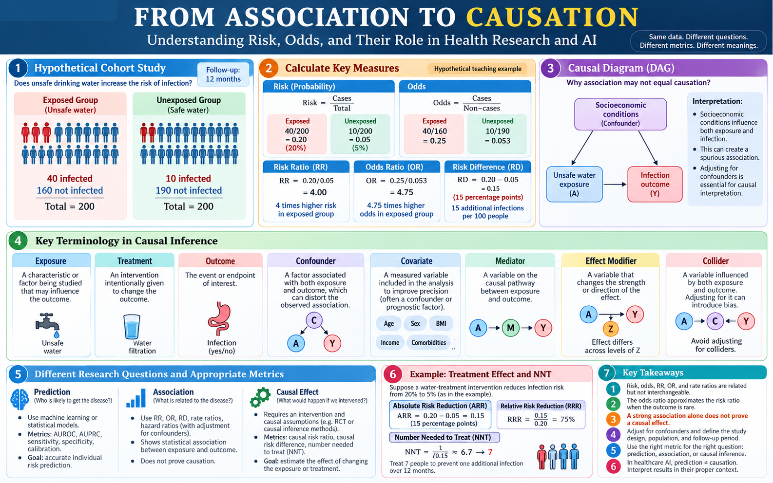
Select the infographic to view it at full size. The treatment-effect calculations refer to the separate hypothetical intervention described in Section 6; the observed cohort association alone does not establish a treatment effect.
References
- Dettori JR, Norvell DC, Chapman JR. Risks, Rates and Odds: What’s the Difference and Why Does It Matter? Global Spine Journal. 2021;11(7):1156–1158. https://doi.org/10.1177/21925682211029640
- Hernán MA, Robins JM. Causal Inference: What If. Chapman & Hall/CRC, 2020. https://www.hsph.harvard.edu/miguel-hernan/wp-content/uploads/sites/1268/2024/04/hernanrobins_WhatIf_26apr24.pdf
- Vandenbroucke JP, von Elm E, Altman DG, et al. Strengthening the Reporting of Observational Studies in Epidemiology (STROBE): Explanation and Elaboration. PLOS Medicine. 2007;4(10):e297. https://doi.org/10.1371/journal.pmed.0040297
- Davies HTO, Crombie IK, Tavakoli M. When can odds ratios mislead? BMJ. 1998;316:989–991. https://doi.org/10.1136/bmj.316.7136.989
- Zhang J, Yu KF. What’s the Relative Risk? A Method of Correcting the Odds Ratio in Cohort Studies of Common Outcomes. JAMA. 1998;280(19):1690–1691. https://doi.org/10.1001/jama.280.19.1690
- Pearl J. Causality: Models, Reasoning, and Inference. 2nd ed. Cambridge University Press, 2009. https://doi.org/10.1017/CBO9780511803161
- Hernán MA. The C-Word: Scientific Euphemisms Do Not Improve Causal Inference From Observational Data. American Journal of Public Health. 2018;108(5):616–619. https://doi.org/10.2105/AJPH.2018.304337