<?xml version="1.0" encoding="utf-8"?><feed xmlns="http://www.w3.org/2005/Atom" ><generator uri="https://jekyllrb.com/" version="3.10.0">Jekyll</generator><link href="https://inamullah-colab.github.io/feed.xml" rel="self" type="application/atom+xml" /><link href="https://inamullah-colab.github.io/" rel="alternate" type="text/html" /><updated>2026-09-14T12:04:08+00:00</updated><id>https://inamullah-colab.github.io/feed.xml</id><title type="html">Inam Ullah Khan</title><subtitle>PhD researcher in oculomics, interpretable machine learning, and multimodal biomedical data integration.</subtitle><author><name>Inam Ullah Khan</name><email>i1n23@soton.ac.uk</email></author><entry><title type="html">From School Formulas to Modern Systems</title><link href="https://inamullah-colab.github.io/posts/2026/07/from-school-formulas-to-modern-systems/" rel="alternate" type="text/html" title="From School Formulas to Modern Systems" /><published>2026-07-14T12:00:00+00:00</published><updated>2026-07-14T12:00:00+00:00</updated><id>https://inamullah-colab.github.io/posts/2026/07/from-school-formulas-to-modern-systems</id><content type="html" xml:base="https://inamullah-colab.github.io/posts/2026/07/from-school-formulas-to-modern-systems/"><![CDATA[<h1 id="from-school-formulas-to-modern-systems">From School Formulas to Modern Systems</h1>

<p>There was a stage in school when I genuinely felt bored by mathematics and physics.</p>

<p>Not because the subjects were unimportant, but because I could not yet see what they were for.</p>

<p>A page filled with angles, trigonometric identities, derivatives, vector operators, and field equations can feel exhausting when all you see is symbolic pressure and no living context. At that age, it is easy to ask:</p>

<blockquote>
  <p>Why am I spending so much time on this?<br />
Where does this appear in practical life?</p>
</blockquote>

<p>At the time, those questions felt reasonable to me. I could solve exercises, but I could not yet see a convincing bridge between formal mathematics and the real world.</p>

<p>What changed later was not the symbols. What changed was my perspective.</p>

<p>Once I moved into scientific computing, image analysis, quantitative modelling, and machine learning, I started to recognise that many of those old formulas were not isolated school tasks at all. They were compact descriptions of mechanisms:</p>

<ul>
  <li>how geometry behaves,</li>
  <li>how signals repeat,</li>
  <li>how fields evolve,</li>
  <li>how nonlinear systems are approximated,</li>
  <li>how uncertainty is represented,</li>
  <li>how models learn from data,</li>
  <li>and how theory becomes something implementable.</li>
</ul>

<p>That is the broader idea behind this post.</p>

<h2 id="the-diagram-as-a-map-not-decoration">The Diagram as a Map, Not Decoration</h2>

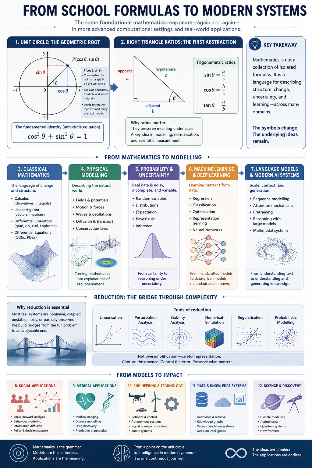
<p>The figure below is meant to do more than look attractive. It is intended to summarise a chain of ideas that often appears fragmented when we first encounter it:</p>

<ul>
  <li>trigonometric ratios and the unit circle,</li>
  <li>classical mathematical structure,</li>
  <li>physical modelling,</li>
  <li>probabilistic reasoning,</li>
  <li>machine learning and deep learning,</li>
  <li>language models and modern computational systems,</li>
  <li>and finally social and medical applications.</li>
</ul>

<div class="math-journey-figure">
  <img src="/images/math-from-school-to-modern-systems.png" alt="Visual map linking the unit circle and trigonometric ratios to classical mathematics, physics, probability, machine learning, language models, and real-world applications." />
</div>

<p>The point of the figure is not to claim that every modern system comes directly from one trigonometric identity. That would be shallow. The point is subtler: the same foundational mathematics keeps reappearing, often under different names, in more advanced computational settings.</p>

<h2 id="why-the-unit-circle-is-more-important-than-it-first-appears">Why the Unit Circle Is More Important Than It First Appears</h2>

<p>For many students, trigonometry begins as memorisation:</p>

\[\sin \theta, \qquad \cos \theta, \qquad \tan \theta.\]

<p>That is often where boredom begins as well. Without a geometric picture, these expressions can feel like arbitrary symbols.</p>

<p>But the unit circle changes the story.</p>

<p>The point at angle $\theta$ is</p>

\[(\cos \theta, \sin \theta).\]

<p>That single statement already explains:</p>

<ul>
  <li>why cosine and sine are coordinates,</li>
  <li>why periodicity emerges naturally,</li>
  <li>why rotation matrices use those functions,</li>
  <li>why circular motion and wave behaviour are mathematically connected.</li>
</ul>

<p>It also makes the classical identity</p>

\[\sin^2 \theta + \cos^2 \theta = 1\]

<p>look much less mysterious, because it is simply the unit-circle equation in disguise.</p>

<p>This is one of the first places where mathematics becomes more meaningful when moved from memorisation into structure.</p>

<h2 id="what-the-triangle-ratios-really-give-us">What the Triangle Ratios Really Give Us</h2>

<p>The familiar right-triangle definitions</p>

\[\sin \theta = \frac{\text{opposite}}{\text{hypotenuse}}, \qquad
\cos \theta = \frac{\text{adjacent}}{\text{hypotenuse}}, \qquad
\tan \theta = \frac{\text{opposite}}{\text{adjacent}}\]

<p>are not just school exercises. They teach an important modelling habit: <strong>ratios can preserve meaning under scale</strong>.</p>

<p>That is already a scientific idea.</p>

<p>When a quantity is written as a ratio rather than a raw magnitude, it often becomes more stable, more transferable, and more interpretable. This is one reason trigonometric thinking survives into signal processing, coordinate systems, numerical geometry, and many imaging tasks.</p>

<p>In practical work, the same mental move happens again and again:</p>

<ul>
  <li>use structure rather than raw values,</li>
  <li>represent behaviour in a normalised form,</li>
  <li>search for invariants that survive scaling, noise, or transformation.</li>
</ul>

<h2 id="from-geometry-to-physical-modelling">From Geometry to Physical Modelling</h2>

<p>At a broader level, mathematical physics often begins by asking:</p>

<ul>
  <li>what is changing,</li>
  <li>where is it changing,</li>
  <li>how fast is it changing,</li>
  <li>in which direction is it changing,</li>
  <li>and what constraints govern that change?</li>
</ul>

<p>That leads naturally to ideas such as:</p>

<ul>
  <li>scalar fields,</li>
  <li>vector fields,</li>
  <li>gradients,</li>
  <li>divergence,</li>
  <li>curl,</li>
  <li>Laplacians.</li>
</ul>

<p>At school, these may appear as formal operations. Later, they become ways of describing very real phenomena:</p>

<ul>
  <li>transport,</li>
  <li>flow,</li>
  <li>accumulation,</li>
  <li>diffusion,</li>
  <li>oscillation,</li>
  <li>potential,</li>
  <li>conservation.</li>
</ul>

<p>The language becomes increasingly expressive. What once looked symbolic begins to function as a modelling grammar.</p>

<h2 id="nonlinearity-and-the-need-for-reduction">Nonlinearity and the Need for Reduction</h2>

<p>One of the hardest transitions in applied mathematics is realising that most important systems are not perfectly simple.</p>

<p>They are often nonlinear, unstable, coupled, noisy, or only partially observed.</p>

<p>This is where a deeper mathematical mindset becomes useful. Instead of asking for one perfect closed-form answer, we begin asking:</p>

<ul>
  <li>Can the system be approximated locally?</li>
  <li>Can a nonlinear phenomenon be studied through linearisation?</li>
  <li>Can we separate dominant structure from noise?</li>
  <li>Can we control sensitivity?</li>
  <li>Can we transform the problem into a tractable form?</li>
</ul>

<p>This is where reduction becomes central.</p>

<p>Reduction does not mean oversimplification. It means building a careful bridge from the full problem to an analysable one.</p>

<p>That same mindset appears in:</p>

<ul>
  <li>local linear approximation,</li>
  <li>perturbation analysis,</li>
  <li>stability studies,</li>
  <li>numerical simulation,</li>
  <li>regularisation,</li>
  <li>probabilistic modelling.</li>
</ul>

<p>Many systems that appear chaotic or entropic at first sight become partially understandable only because we learn how to represent them in a better mathematical language.</p>

<h2 id="why-probability-enters-the-story">Why Probability Enters the Story</h2>

<p>Pure geometry and deterministic physics are powerful, but real data rarely arrive in clean exact form.</p>

<p>Measurements are noisy. Observations are incomplete. Biological systems vary. Sensors fail. Human behaviour is irregular. Real-world systems contain uncertainty by default.</p>

<p>That is why probability becomes unavoidable.</p>

<p>Probability gives us a disciplined language for:</p>

<ul>
  <li>uncertainty,</li>
  <li>variability,</li>
  <li>inference,</li>
  <li>confidence,</li>
  <li>noise modelling,</li>
  <li>prediction under partial information.</li>
</ul>

<p>This is not separate from the rest of mathematics. It is what allows structural mathematics to survive contact with imperfect reality.</p>

<p>In practice, many useful models stand at the intersection of:</p>

<ul>
  <li>geometric structure,</li>
  <li>physical intuition,</li>
  <li>probabilistic uncertainty,</li>
  <li>computational approximation.</li>
</ul>

<p>That intersection is where a large part of modern quantitative science actually lives.</p>

<h2 id="the-bridge-to-machine-learning">The Bridge to Machine Learning</h2>

<p>Machine learning often appears modern and self-contained, but it is built from older mathematical layers.</p>

<p>At a minimum, it depends on:</p>

<ul>
  <li><strong>linear algebra</strong> for representation and transformation,</li>
  <li><strong>calculus</strong> for gradients and optimisation,</li>
  <li><strong>probability</strong> for uncertainty and statistical learning,</li>
  <li><strong>geometry</strong> for similarity, embeddings, and structure,</li>
  <li><strong>approximation theory</strong> for generalisation and expressive modelling.</li>
</ul>

<p>Even deep learning, which is nonlinear overall, is still assembled from repeated linear maps plus nonlinear activation functions and optimised through gradient-based updates.</p>

<p>That is why I no longer see older mathematics as “before AI” knowledge. It is still inside AI.</p>

<h2 id="deep-learning-and-foundation-models">Deep Learning and Foundation Models</h2>

<p>When people speak about deep learning, language models, or ChatGPT-style systems, the surface looks very different from school mathematics. The interface is fluent and conversational. The user does not see the mathematics directly.</p>

<p>But beneath that surface, the chain still holds:</p>

<ul>
  <li>vectors,</li>
  <li>matrices,</li>
  <li>dot products,</li>
  <li>probabilistic outputs,</li>
  <li>optimisation,</li>
  <li>representation learning.</li>
</ul>

<p>Language models extend this into large-scale sequence modelling, contextual embeddings, attention mechanisms, and token prediction, but they are still mathematical systems before they are interface systems.</p>

<p>This matters because it prevents us from mystifying the technology. We can admire the scale and sophistication without forgetting that structure, approximation, and optimisation still govern the result.</p>

<h2 id="why-this-matters-in-social-and-medical-settings">Why This Matters in Social and Medical Settings</h2>

<p>For me, the most meaningful shift happened when I started seeing how these mathematical ideas move into domains that affect real lives.</p>

<p>In social systems, they can support:</p>

<ul>
  <li>forecasting,</li>
  <li>decision support,</li>
  <li>behavioural pattern analysis,</li>
  <li>risk-aware modelling.</li>
</ul>

<p>In medical and biomedical settings, they can support:</p>

<ul>
  <li>image interpretation,</li>
  <li>signal analysis,</li>
  <li>disease modelling,</li>
  <li>biomarker discovery,</li>
  <li>uncertainty-aware decision systems.</li>
</ul>

<p>That final step matters.</p>

<p>A formula becomes much more meaningful once it participates in a chain that runs from theory to an interpretable real-world outcome. In biomedical research especially, the path often looks something like this:</p>

<ol>
  <li>start from assumptions,</li>
  <li>define a mathematical model,</li>
  <li>derive or justify its structure,</li>
  <li>simulate or estimate behaviour,</li>
  <li>test it on data,</li>
  <li>interpret it cautiously,</li>
  <li>decide whether it is trustworthy enough to matter.</li>
</ol>

<p>This is where mathematics stops being an isolated subject and becomes part of scientific responsibility.</p>

<h2 id="what-i-understand-differently-now">What I Understand Differently Now</h2>

<p>When I was younger, I thought mathematics and physics were mostly about solving problems correctly.</p>

<p>Now I see them more as a layered framework for thought:</p>

<ul>
  <li>notation,</li>
  <li>assumption,</li>
  <li>abstraction,</li>
  <li>reduction,</li>
  <li>theorem,</li>
  <li>proof,</li>
  <li>simulation,</li>
  <li>implementation,</li>
  <li>application.</li>
</ul>

<p>That sequence is not always linear, but it is one of the clearest ways I now understand how theory becomes practice.</p>

<p>The older formulas did not lose their relevance. I simply reached the stage where I could finally see what they were supporting.</p>

<h2 id="final-reflection">Final Reflection</h2>

<p>I do not think every student must immediately love mathematics or physics. Confusion and boredom are real experiences. I had them too.</p>

<p>But I now think many of those early formulas deserve more respect than they often receive, because they are not merely decorative pieces of a syllabus. They are part of a long intellectual infrastructure that supports scientific explanation, computational reasoning, and practical systems.</p>

<p>Some of that infrastructure begins with a triangle.<br />
Some of it begins with a circle.<br />
Some of it appears in a gradient, a divergence, a curl, or a Laplacian.<br />
Some of it appears in probability and inference.<br />
Some of it appears in machine learning, deep learning, and language models.<br />
And some of it returns, eventually, to human questions in medicine and society.</p>

<p>That is why I no longer see those old school formulas as time wasted.</p>

<p>I see them as the early pieces of a much larger map.</p>]]></content><author><name>Inam Ullah Khan</name><email>i1n23@soton.ac.uk</email></author><category term="mathematics" /><category term="trigonometry" /><category term="physics" /><category term="probability" /><category term="vector-calculus" /><category term="machine-learning" /><category term="deep-learning" /><category term="scientific-computing" /><summary type="html"><![CDATA[A detailed reflection on how the formulas that once felt empty at school later became part of the practical language of modelling, proof, simulation, machine learning, and medical applications.]]></summary></entry><entry><title type="html">Five Constants, One Truth: Euler’s Identity, A Deeper Look</title><link href="https://inamullah-colab.github.io/posts/2026/04/five-constants-one-truth-eulers-identity-deeper-look/" rel="alternate" type="text/html" title="Five Constants, One Truth: Euler’s Identity, A Deeper Look" /><published>2026-04-19T12:00:00+00:00</published><updated>2026-04-19T12:00:00+00:00</updated><id>https://inamullah-colab.github.io/posts/2026/04/five-constants-one-truth-eulers-identity-deeper-look</id><content type="html" xml:base="https://inamullah-colab.github.io/posts/2026/04/five-constants-one-truth-eulers-identity-deeper-look/"><![CDATA[<h1 id="the-most-beautiful-equation-in-mathematics">The Most Beautiful Equation in Mathematics</h1>

<p>Few equations are as compact, famous, and conceptually rich as Euler’s identity:</p>

\[e^{i\pi}+1=0\]

<p>Equivalently,</p>

\[e^{i\pi}=-1\]

<p>In a single line, this equation brings together five of the most important constants in mathematics:</p>

<ul>
  <li>$0$, the additive identity</li>
  <li>$1$, the multiplicative identity</li>
  <li>$\pi$, the circle constant</li>
  <li>$e$, the base of natural logarithms</li>
  <li>$i$, the imaginary unit</li>
</ul>

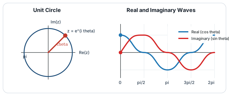
<p>That is one reason the formula is so admired. It does not merely look elegant. It reveals an unexpected connection between ideas that first arise in very different parts of mathematics: arithmetic, geometry, algebra, and analysis.<sup id="fnref:1" role="doc-noteref"><a href="#fn:1" class="footnote" rel="footnote">1</a></sup></p>

<div class="euler-figure">
  <img src="/images/euler-waves-animated.svg" alt="Animated Euler diagram showing the unit circle together with the real cosine wave and the imaginary sine wave" />
</div>

<h2 id="eulers-formula-comes-first">Euler’s Formula Comes First</h2>

<p>To understand Euler’s identity properly, it helps to distinguish <strong>Euler’s formula</strong> from <strong>Euler’s identity</strong>.</p>

<p>Euler’s formula is</p>

\[e^{i\theta}=\cos\theta+i\sin\theta\]

<p>Euler’s identity is the special case obtained by setting $\theta=\pi$:</p>

\[e^{i\pi}=\cos\pi+i\sin\pi=-1+0i=-1\]

<p>so</p>

\[e^{i\pi}+1=0\]

<p>This means Euler’s identity is not an isolated miracle. It is a particularly beautiful consequence of a deeper and more general relationship between exponentials and trigonometric functions.<sup id="fnref:1:1" role="doc-noteref"><a href="#fn:1" class="footnote" rel="footnote">1</a></sup></p>

<h2 id="a-short-derivation">A Short Derivation</h2>

<p>One clean way to see why Euler’s formula is true is through the power series for the exponential, cosine, and sine functions:</p>

\[e^x=\sum_{n=0}^{\infty}\frac{x^n}{n!}, \qquad
\cos x=\sum_{k=0}^{\infty}\frac{(-1)^k x^{2k}}{(2k)!}, \qquad
\sin x=\sum_{k=0}^{\infty}\frac{(-1)^k x^{2k+1}}{(2k+1)!}\]

<p>Now replace $x$ by $i\theta$ in the exponential series:</p>

\[e^{i\theta}
= \sum_{n=0}^{\infty}\frac{(i\theta)^n}{n!}
= 1+i\theta+\frac{(i\theta)^2}{2!}+\frac{(i\theta)^3}{3!}+\cdots\]

<p>Using the fact that powers of $i$ cycle as</p>

\[i^0=1,\quad i^1=i,\quad i^2=-1,\quad i^3=-i,\quad i^4=1,\]

<p>the even and odd terms separate naturally into real and imaginary parts:</p>

\[e^{i\theta}
= \left(1-\frac{\theta^2}{2!}+\frac{\theta^4}{4!}-\cdots\right)
+ i\left(\theta-\frac{\theta^3}{3!}+\frac{\theta^5}{5!}-\cdots\right)\]

<p>which is exactly</p>

\[e^{i\theta}=\cos\theta+i\sin\theta\]

<p>Setting $\theta=\pi$ gives</p>

\[e^{i\pi}=\cos\pi+i\sin\pi=-1\]

<p>and therefore</p>

\[e^{i\pi}+1=0\]

<p>For many readers, this is the moment where the equation stops being mysterious and starts becoming profound.</p>

<h2 id="the-five-constants">The Five Constants</h2>

<h3 id="0-the-additive-identity">$0$: The Additive Identity</h3>

<p>Zero represents the neutral element of addition. For any number $a$,</p>

\[a+0=a\]

<p>It is hard to imagine modern mathematics, algebra, or computation without zero. It is both a number and a structural idea: the reference point from which positive and negative quantities are measured.</p>

<h3 id="1-the-multiplicative-identity">$1$: The Multiplicative Identity</h3>

<p>One is the neutral element of multiplication. For any number $a$,</p>

\[a\cdot 1=a\]

<p>Like zero, it seems simple, but it plays a foundational role. In algebraic structures, identities are what let operations hold together coherently.</p>

<h3 id="pi-the-circle-constant">$\pi$: The Circle Constant</h3>

<p>$\pi$ is the ratio of a circle’s circumference to its diameter:</p>

\[\pi=\frac{C}{D}\]

<p>It appears not only in geometry, but throughout calculus, differential equations, Fourier analysis, probability, and physics. It is irrational and transcendental, so its decimal expansion never terminates and never repeats.<sup id="fnref:1:2" role="doc-noteref"><a href="#fn:1" class="footnote" rel="footnote">1</a></sup></p>

<h3 id="e-the-growth-constant">$e$: The Growth Constant</h3>

<p>The constant $e$ arises naturally in continuous growth, compound interest, and differential equations. It is the base of the natural logarithm and the unique number for which the derivative of $e^x$ is itself:</p>

\[\frac{d}{dx}e^x=e^x\]

<p>That property makes $e$ fundamental in continuous-time mathematics.<sup id="fnref:1:3" role="doc-noteref"><a href="#fn:1" class="footnote" rel="footnote">1</a></sup></p>

<h3 id="i-the-imaginary-unit">$i$: The Imaginary Unit</h3>

<p>The imaginary unit is defined by</p>

\[i^2=-1\]

<p>This does not make it unreal. It extends the real number system into the complex plane, where numbers can encode both magnitude and direction. Complex numbers are essential in wave theory, circuit analysis, quantum mechanics, and signal processing.<sup id="fnref:2" role="doc-noteref"><a href="#fn:2" class="footnote" rel="footnote">2</a></sup><sup id="fnref:3" role="doc-noteref"><a href="#fn:3" class="footnote" rel="footnote">3</a></sup></p>

<h2 id="the-geometric-meaning-rotation-on-the-complex-plane">The Geometric Meaning: Rotation on the Complex Plane</h2>

<p>Euler’s formula becomes especially intuitive when viewed geometrically.</p>

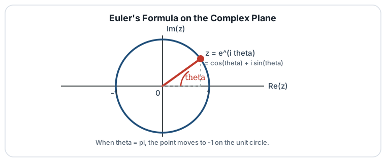
<p>A complex number can be represented as a point on the complex plane, with the horizontal axis as the real part and the vertical axis as the imaginary part. According to</p>

\[e^{i\theta}=\cos\theta+i\sin\theta,\]

<p>the number $e^{i\theta}$ lies on the unit circle at angle $\theta$.</p>

<p>So when $\theta=\pi$, the point lies exactly halfway around the circle from $1$, landing at $-1$:</p>

\[e^{i\pi}=-1\]

<p>This is why Euler’s identity can be interpreted as a perfect half-turn. The exponential expression does not merely “grow”; in the complex setting, it rotates.</p>

<div class="euler-figure">
  <img src="/images/euler-unit-circle.svg" alt="Unit circle interpretation of Euler's formula showing e^(i theta) as a point at angle theta on the complex plane" />
</div>

<h2 id="a-simple-analogy">A Simple Analogy</h2>

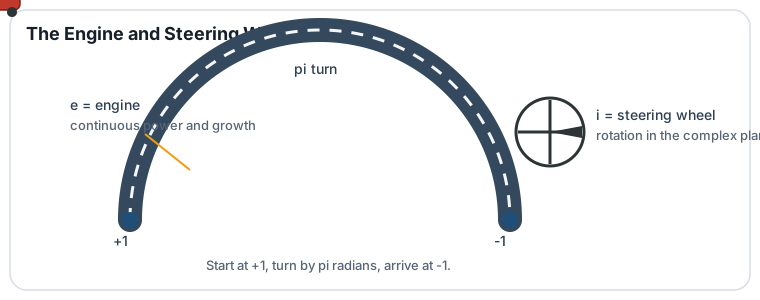
<p>A good analogy is to think of the formula as combining <strong>motion</strong> and <strong>direction</strong>.</p>

<ul>
  <li>$e$ captures the exponential structure</li>
  <li>$i$ introduces rotation into the complex plane</li>
  <li>$\pi$ specifies the exact angle: half a turn</li>
  <li>the result is $-1$, the point directly opposite $+1$</li>
  <li>adding $1$ returns the balance point $0$</li>
</ul>

<p>This analogy should not be taken as a proof, but it is helpful intuition. Euler’s identity says that exponential structure and circular motion are not separate ideas. They fit into one framework.</p>

<div class="euler-figure">
  <img src="/images/euler-engine-steering-animated.svg" alt="Animated engine and steering wheel analogy for Euler's identity" />
</div>

<h2 id="why-physicists-and-engineers-care">Why Physicists and Engineers Care</h2>

<p>The importance of Euler’s formula extends far beyond pure mathematics.</p>

<p>In engineering and physics, oscillations are often written in the form</p>

\[e^{i\omega t}\]

<p>where $\omega$ is angular frequency and $t$ is time. By Euler’s formula,</p>

\[e^{i\omega t}=\cos(\omega t)+i\sin(\omega t)\]

<p>This compact form lets one represent sinusoidal motion, phase, and frequency in a single expression. That is why complex exponentials are standard in:</p>

<ul>
  <li>alternating current circuit analysis</li>
  <li>wave propagation</li>
  <li>electromagnetism</li>
  <li>control systems</li>
  <li>quantum mechanics</li>
  <li>signal processing<sup id="fnref:2:1" role="doc-noteref"><a href="#fn:2" class="footnote" rel="footnote">2</a></sup><sup id="fnref:3:1" role="doc-noteref"><a href="#fn:3" class="footnote" rel="footnote">3</a></sup></li>
</ul>

<p>In practice, the real and imaginary parts encode cosine-like and sine-like components. Engineers often compute with the compact exponential form first and then extract the physically meaningful real part afterward.</p>

<h2 id="why-it-matters-in-statistics-and-data-analysis">Why It Matters in Statistics and Data Analysis</h2>

<p>The mathematics behind Euler’s formula also appears in probability and data analysis.</p>

<h3 id="fourier-analysis">Fourier analysis</h3>

<p>A core tool in signal analysis is the decomposition of a signal into frequency components. In discrete form, the key kernel is</p>

\[e^{-2\pi i kn/N}\]

<p>This is the mathematical backbone of Fourier methods, which are used to detect periodic structure, filter signals, compress information, and analyze time-series data.<sup id="fnref:2:2" role="doc-noteref"><a href="#fn:2" class="footnote" rel="footnote">2</a></sup></p>

<h3 id="characteristic-functions-in-probability">Characteristic functions in probability</h3>

<p>In probability theory, the characteristic function of a random variable $X$ is</p>

\[\varphi_X(t)=\mathbb{E}[e^{itX}]\]

<p>This is one of the most important bridges between probability and harmonic analysis. It encodes the distribution of a random variable in a form that is often easier to manipulate analytically.<sup id="fnref:4" role="doc-noteref"><a href="#fn:4" class="footnote" rel="footnote">4</a></sup></p>

<h3 id="circular-statistics">Circular statistics</h3>

<p>Whenever data are angular rather than linear, such as directions, phases, or times of day on a cycle, complex exponentials become natural tools. Circular statistics often uses the representation</p>

\[e^{i\theta}\]

<p>because it respects the geometry of angles in a way that ordinary linear statistics does not.<sup id="fnref:5" role="doc-noteref"><a href="#fn:5" class="footnote" rel="footnote">5</a></sup></p>

<h3 id="spectral-structure-and-eigendecomposition">Spectral structure and eigendecomposition</h3>

<p>Complex numbers also appear when linear systems are analyzed through eigenvalues, eigenvectors, and spectral decompositions. Even when the data themselves are real-valued, the mathematics of oscillation and repeated transformation often leads naturally to complex-valued analysis.</p>

<h2 id="what-about-computing-and-ai">What About Computing and AI?</h2>

<p>This part needs careful wording.</p>

<p>Euler’s identity itself is not explicitly used in most machine-learning models. However, the broader mathematics behind it, especially complex exponentials, trigonometric structure, and Fourier analysis, appears in several computational settings.</p>

<p>Examples include:</p>

<ul>
  <li>frequency-domain signal processing</li>
  <li>audio and speech analysis</li>
  <li>scientific computing</li>
  <li>Fourier-based feature mappings</li>
  <li>some symmetry-aware and equivariant models</li>
  <li>quantum information and quantum computing<sup id="fnref:2:3" role="doc-noteref"><a href="#fn:2" class="footnote" rel="footnote">2</a></sup><sup id="fnref:6" role="doc-noteref"><a href="#fn:6" class="footnote" rel="footnote">6</a></sup><sup id="fnref:7" role="doc-noteref"><a href="#fn:7" class="footnote" rel="footnote">7</a></sup></li>
</ul>

<p>A more accurate statement is this:</p>

<blockquote>
  <p>Euler’s identity is not “the formula behind all AI,” but the mathematics surrounding Euler’s formula plays an important role in several areas of modern computation.</p>
</blockquote>

<p>That phrasing is both stronger and more scientifically honest.</p>

<h2 id="why-people-find-it-beautiful">Why People Find It Beautiful</h2>

<p>Euler’s identity is often described as beautiful because it compresses a surprising amount of mathematics into one exact statement.</p>

<p>It connects:</p>

<ol>
  <li>arithmetic identities through $0$ and $1$</li>
  <li>geometry through $\pi$</li>
  <li>analysis through $e$</li>
  <li>algebra through $i$</li>
  <li>structure and symmetry through the complex plane</li>
</ol>

<p>Its beauty is not only that it is short. It is that it feels inevitable once understood, even though it looks impossible at first glance.</p>

<h2 id="a-final-reflection">A Final Reflection</h2>

<p>Euler’s identity is a reminder that mathematics is full of hidden unity. Ideas that begin in separate chapters of a textbook often turn out to be aspects of the same deeper structure.</p>

<p>What starts as a formula about exponentials becomes a statement about rotation.<br />
What begins in pure mathematics becomes a working language for waves, signals, probability, and computation.</p>

<p>That is why</p>

\[e^{i\pi}+1=0\]

<p>continues to fascinate students, scientists, and mathematicians alike. It is not just a clever equation. It is a compact window into how different parts of mathematics fit together.</p>

<hr />

<h2 id="references">References</h2>

<div class="footnotes" role="doc-endnotes">
  <ol>
    <li id="fn:1" role="doc-endnote">
      <p>NIST Digital Library of Mathematical Functions, Chapter 4: <em>Elementary Functions</em>. <a href="#fnref:1" class="reversefootnote" role="doc-backlink">&#8617;</a> <a href="#fnref:1:1" class="reversefootnote" role="doc-backlink">&#8617;<sup>2</sup></a> <a href="#fnref:1:2" class="reversefootnote" role="doc-backlink">&#8617;<sup>3</sup></a> <a href="#fnref:1:3" class="reversefootnote" role="doc-backlink">&#8617;<sup>4</sup></a></p>
    </li>
    <li id="fn:2" role="doc-endnote">
      <p>Alan V. Oppenheim and Ronald W. Schafer, <em>Discrete-Time Signal Processing</em>. <a href="#fnref:2" class="reversefootnote" role="doc-backlink">&#8617;</a> <a href="#fnref:2:1" class="reversefootnote" role="doc-backlink">&#8617;<sup>2</sup></a> <a href="#fnref:2:2" class="reversefootnote" role="doc-backlink">&#8617;<sup>3</sup></a> <a href="#fnref:2:3" class="reversefootnote" role="doc-backlink">&#8617;<sup>4</sup></a></p>
    </li>
    <li id="fn:3" role="doc-endnote">
      <p>David J. Griffiths and Darrell F. Schroeter, <em>Introduction to Quantum Mechanics</em>. <a href="#fnref:3" class="reversefootnote" role="doc-backlink">&#8617;</a> <a href="#fnref:3:1" class="reversefootnote" role="doc-backlink">&#8617;<sup>2</sup></a></p>
    </li>
    <li id="fn:4" role="doc-endnote">
      <p>Eugene Lukacs, <em>Characteristic Functions</em>. <a href="#fnref:4" class="reversefootnote" role="doc-backlink">&#8617;</a></p>
    </li>
    <li id="fn:5" role="doc-endnote">
      <p>Kanti V. Mardia and Peter E. Jupp, <em>Directional Statistics</em>. <a href="#fnref:5" class="reversefootnote" role="doc-backlink">&#8617;</a></p>
    </li>
    <li id="fn:6" role="doc-endnote">
      <p>Ronald N. Bracewell, <em>The Fourier Transform and Its Applications</em>. <a href="#fnref:6" class="reversefootnote" role="doc-backlink">&#8617;</a></p>
    </li>
    <li id="fn:7" role="doc-endnote">
      <p>Matthew Tancik et al., “Fourier Features Let Networks Learn High Frequency Functions in Low Dimensional Domains.” <a href="#fnref:7" class="reversefootnote" role="doc-backlink">&#8617;</a></p>
    </li>
  </ol>
</div>]]></content><author><name>Inam Ullah Khan</name><email>i1n23@soton.ac.uk</email></author><category term="mathematics" /><category term="euler" /><category term="complex-numbers" /><category term="physics" /><category term="signal-processing" /><category term="computing" /><summary type="html"><![CDATA[Euler's identity, e^{i\pi}+1=0, links five fundamental constants in one compact equation and opens a doorway to complex numbers, geometry, waves, and modern computation.]]></summary></entry><entry><title type="html">AutoMorph from Local Repo to HPC/SSH: one definitive guide</title><link href="https://inamullah-colab.github.io/automorph-local-and-hpc/" rel="alternate" type="text/html" title="AutoMorph from Local Repo to HPC/SSH: one definitive guide" /><published>2026-02-15T00:00:00+00:00</published><updated>2026-02-15T00:00:00+00:00</updated><id>https://inamullah-colab.github.io/automorph-oculomics-hpc-guide</id><content type="html" xml:base="https://inamullah-colab.github.io/automorph-local-and-hpc/"><![CDATA[<style>
.automorph-page {
  --bg1: #f0f9ff;
  --bg2: #f7fee7;
  --ink: #0f172a;
  --muted: #334155;
  --primary: #0ea5e9;
  --secondary: #22c55e;
  --card: #ffffff;
  --ring: rgba(14, 165, 233, 0.18);
  color: var(--ink);
  font-family: "Segoe UI", "Trebuchet MS", Helvetica, Arial, sans-serif;
}

.automorph-hero {
  background: linear-gradient(135deg, #0ea5e9 0%, #22c55e 100%);
  color: #ffffff;
  border-radius: 18px;
  padding: 28px;
  box-shadow: 0 12px 30px rgba(2, 132, 199, 0.22);
  margin: 12px 0 22px 0;
}

.automorph-hero h1 {
  margin: 0 0 10px 0;
  line-height: 1.2;
  font-size: clamp(1.4rem, 2.2vw, 2rem);
}

.automorph-hero p {
  margin: 8px 0 0 0;
  opacity: 0.98;
}

.automorph-grid {
  display: grid;
  grid-template-columns: repeat(auto-fit, minmax(220px, 1fr));
  gap: 12px;
  margin: 16px 0 22px 0;
}

.automorph-chip {
  background: #ecfeff;
  border: 1px solid #bae6fd;
  border-radius: 12px;
  padding: 10px 12px;
  font-size: 0.93rem;
  color: #075985;
}

.automorph-section {
  background: linear-gradient(180deg, var(--card), #f8fafc);
  border: 1px solid #e2e8f0;
  border-radius: 14px;
  padding: 18px;
  margin: 14px 0;
  box-shadow: 0 3px 14px rgba(15, 23, 42, 0.06);
}

.automorph-section h2 {
  margin-top: 0;
  border-left: 5px solid var(--primary);
  padding-left: 10px;
}

.automorph-callout {
  border-left: 5px solid var(--secondary);
  background: #f0fdf4;
  border-radius: 10px;
  padding: 12px 14px;
  margin: 10px 0;
  color: #14532d;
}

.automorph-page ul {
  margin-top: 8px;
}

.automorph-page pre {
  background: #0b1020;
  color: #dbeafe;
  border-radius: 12px;
  padding: 12px;
  overflow-x: auto;
  border: 1px solid #1e293b;
  box-shadow: inset 0 0 0 1px rgba(148, 163, 184, 0.12);
}

.automorph-page code {
  font-family: Consolas, "Courier New", monospace;
}

.automorph-page pre code {
  color: #f8fafc !important;
  opacity: 1;
}

.automorph-kpis {
  display: grid;
  grid-template-columns: repeat(auto-fit, minmax(150px, 1fr));
  gap: 10px;
  margin: 12px 0 0 0;
}

.automorph-kpi {
  background: #ffffff;
  border: 1px solid #d1fae5;
  border-radius: 10px;
  padding: 10px;
}

.automorph-kpi b {
  display: block;
  font-size: 1.05rem;
  color: #065f46;
}

.automorph-refs a {
  word-break: break-word;
}
</style>

<div class="automorph-page">
  <section class="automorph-hero">
    <h1>AutoMorph from Local Repo to HPC/SSH</h1>
    <p>One reproducible, publication-ready workflow for running the official M0-M3 pipeline at small or large scale.</p>
  </section>

  <div class="automorph-grid">
    <div class="automorph-chip"><b>Local path:</b> quick setup, debugging, smaller batches</div>
    <div class="automorph-chip"><b>HPC path:</b> scalable runs, cleaner data separation, long jobs</div>
    <div class="automorph-chip"><b>Calibration:</b> use <code>resolution_information.csv</code> for micron units</div>
    <div class="automorph-chip"><b>Orchestration:</b> <code>run.sh</code> executes M0 to M3 in fixed order</div>
  </div>

  <section class="automorph-section">
    <h2>1) What AutoMorph does</h2>
    <p><b>AutoMorph</b> is an open pipeline for color fundus photographs that generates quantitative retinal phenotypes.</p>
    <ul>
      <li><b>M0</b>: preprocessing</li>
      <li><b>M1</b>: image quality grading</li>
      <li><b>M2</b>: vessel, artery-vein, and disc-cup segmentation</li>
      <li><b>M3</b>: feature extraction for disc-centred, macular Zone B/C, and whole-image regions</li>
    </ul>
    <div class="automorph-kpis">
      <div class="automorph-kpi"><b>M0</b>Input standardization</div>
      <div class="automorph-kpi"><b>M1</b>Gradable subset</div>
      <div class="automorph-kpi"><b>M2</b>Segmentation masks</div>
      <div class="automorph-kpi"><b>M3</b>CSV phenotypes</div>
    </div>
  </section>

  <section class="automorph-section">
    <h2>2) Local setup (official pattern)</h2>
    <p>Use the maintainer guide: <a href="https://github.com/rmaphoh/AutoMorph/blob/main/LOCAL.md">LOCAL.md</a>.</p>
    <pre><code class="language-bash">conda update conda
conda create -n automorph python=3.11 -y
conda activate automorph
git clone https://github.com/rmaphoh/AutoMorph.git
cd AutoMorph

conda install pytorch==2.3.1 torchvision==0.18.1 torchaudio==2.3.1 pytorch-cuda=12.1 -c pytorch -c nvidia -y
pip install --ignore-installed certifi
pip install -r requirement.txt
pip install efficientnet_pytorch==0.7.1 --no-deps</code></pre>
    <p>Place images in <code>images/</code>, provide <code>resolution_information.csv</code>, then run:</p>
    <pre><code class="language-bash">sh run.sh</code></pre>
  </section>

  <section class="automorph-section">
    <h2>3) HPC/SSH setup (recommended for scale)</h2>
    <pre><code class="language-bash">git clone https://github.com/rmaphoh/AutoMorph.git
cd AutoMorph
conda create -n automorph python=3.11 -y
conda activate automorph
pip install -r requirement.txt</code></pre>

    <p>Keep data outside the repository:</p>
    <pre><code class="language-bash">mkdir -p $HOME/retina_all/images
export AUTOMORPH_DATA=$HOME/retina_all</code></pre>

    <p>Generate spacing file for micron calibration:</p>
    <pre><code class="language-bash">python generate_resolution.py 0.008</code></pre>

    <p>Run detached over SSH:</p>
    <pre><code class="language-bash">nohup bash run.sh &gt; "$AUTOMORPH_DATA/automorph_run_$(date +%F_%H%M).log" 2&gt;&amp;1 &amp; disown
tail -f "$AUTOMORPH_DATA"/automorph_run_*.log</code></pre>

    <div class="automorph-callout">
      <b>Important:</b> <code>run.sh</code> cleans <code>Results/</code> at start. Run one job per data root at a time.
    </div>
  </section>

  <section class="automorph-section">
    <h2>4) Expected outputs and verification</h2>
    <pre><code class="language-text">$AUTOMORPH_DATA/
├── images/
├── resolution_information.csv
└── Results/
    ├── M1/
    │   ├── results_ensemble.csv
    │   └── Good_quality/
    ├── M2/
    │   ├── Vessel_binary/
    │   ├── Artery_vein/
    │   └── Disc_cup/
    └── M3/
        ├── Disc_centred/*.csv
        ├── Macular_centred/
        │   ├── Macular_Zone_B_Measurement.csv
        │   └── Macular_Zone_C_Measurement.csv
        └── Whole_image/*.csv</code></pre>

    <pre><code class="language-bash">ls -1 "$AUTOMORPH_DATA/Results/M1/Good_quality" | wc -l
find "$AUTOMORPH_DATA/Results/M2" -maxdepth 2 -type f | head -n 20
find "$AUTOMORPH_DATA/Results/M3" -maxdepth 2 -type f -name '*.csv' | sort</code></pre>
  </section>

  <section class="automorph-section">
    <h2>5) Reproducibility checklist</h2>
    <ul>
      <li>AutoMorph commit hash and run date</li>
      <li>Python, PyTorch, CUDA versions</li>
      <li>GPU model and driver details</li>
      <li><code>AUTOMORPH_DATA</code> path used at runtime</li>
      <li>Resolution source used in <code>resolution_information.csv</code></li>
      <li>Total input images and M1 gradable count</li>
    </ul>
  </section>

  <section class="automorph-section">
    <h2>6) Copy-ready methods text</h2>
    <div class="automorph-callout">
      We used AutoMorph to extract retinal vascular phenotypes from color fundus images. The official <code>run.sh</code> orchestrator was executed from M0 to M3 (preprocessing, quality grading, vessel/artery-vein/disc-cup segmentation, and feature extraction for disc-centred, macular Zone B, macular Zone C, and whole-image regions). Pixel resolution was provided through <code>resolution_information.csv</code>, generated with <code>generate_resolution.py</code> when per-image metadata were unavailable.
    </div>
  </section>

  <section class="automorph-section automorph-refs">
    <h2>7) Authoritative references</h2>
    <ul>
      <li>AutoMorph project page: <a href="https://rmaphoh.github.io/projects/automorph.html">https://rmaphoh.github.io/projects/automorph.html</a></li>
      <li>AutoMorph GitHub repository: <a href="https://github.com/rmaphoh/AutoMorph">https://github.com/rmaphoh/AutoMorph</a></li>
      <li>Local setup guide (<code>LOCAL.md</code>): <a href="https://github.com/rmaphoh/AutoMorph/blob/main/LOCAL.md">https://github.com/rmaphoh/AutoMorph/blob/main/LOCAL.md</a></li>
      <li>Pipeline runner (<code>run.sh</code>): <a href="https://github.com/rmaphoh/AutoMorph/blob/main/run.sh">https://github.com/rmaphoh/AutoMorph/blob/main/run.sh</a></li>
      <li>TVST 2022 paper: <a href="https://tvst.arvojournals.org/article.aspx?articleid=2783477">https://tvst.arvojournals.org/article.aspx?articleid=2783477</a></li>
      <li>medRxiv preprint: <a href="https://www.medrxiv.org/content/10.1101/2022.05.26.22274795v1">https://www.medrxiv.org/content/10.1101/2022.05.26.22274795v1</a></li>
    </ul>
  </section>
</div>]]></content><author><name>Inamullah Inamullah</name></author><category term="AutoMorph" /><category term="oculomics" /><category term="deep learning" /><category term="fundus" /><category term="pipeline" /><category term="HPC" /><category term="SSH" /><category term="local setup" /><summary type="html"><![CDATA[A detailed, reproducible guide to run the official AutoMorph pipeline locally or on HPC/SSH, with validated setup steps, resolution calibration, outputs, quality controls, and publication-ready reporting.]]></summary></entry><entry><title type="html">Scientific and Mathematical Foundations: Formulas I Once Memorised, Then Finally Understood</title><link href="https://inamullah-colab.github.io/foundations/mathematics/scientific-computing/scientific-math-foundations/" rel="alternate" type="text/html" title="Scientific and Mathematical Foundations: Formulas I Once Memorised, Then Finally Understood" /><published>2026-02-08T00:00:00+00:00</published><updated>2026-02-08T00:00:00+00:00</updated><id>https://inamullah-colab.github.io/foundations/mathematics/scientific-computing/scientific-math-foundations</id><content type="html" xml:base="https://inamullah-colab.github.io/foundations/mathematics/scientific-computing/scientific-math-foundations/"><![CDATA[<h2 id="a-school-time-memory">A School-Time Memory</h2>

<p>When I was at school, I often looked at pages full of formulas and thought:</p>

<blockquote>
  <p>Why am I memorising this? What is it actually for?</p>
</blockquote>

<p>At the time, the symbols felt detached from reality. They looked like exercises for passing exams, not tools for understanding anything meaningful.</p>

<p>That changed later.</p>

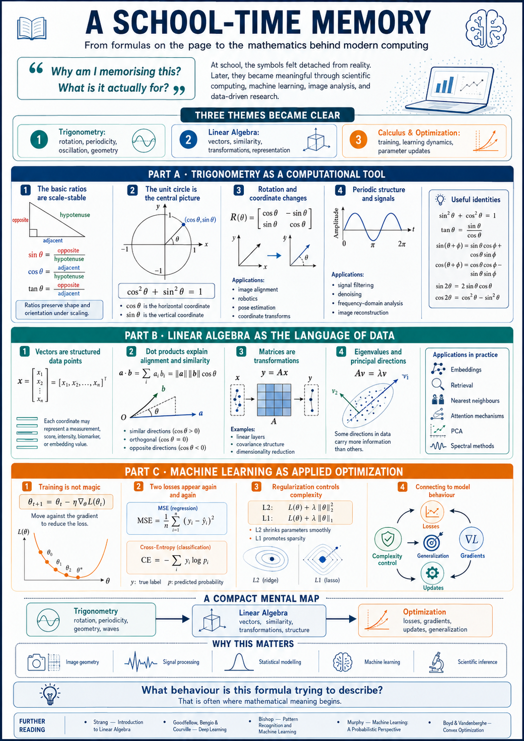
<p>As I moved into scientific computing, machine learning, image analysis, and data-driven research, I began to see that many of those same formulas were not academic ornaments at all. They were compact descriptions of how computation, geometry, signals, and learning behave.</p>

<p>Three themes became especially clear:</p>

<ul>
  <li><strong>Trigonometry</strong> explains rotation, periodicity, oscillation, and geometry.</li>
  <li><strong>Linear algebra</strong> explains vectors, similarity, transformations, and data representation.</li>
  <li><strong>Calculus and optimization</strong> explain training, learning dynamics, and parameter updates.</li>
</ul>

<p>These are not just school topics. They are part of the working language of modern science and computing.</p>

<div class="math-journey-figure">
  <img src="/images/scientific-math-foundations.png" alt="Infographic summarising how trigonometry, linear algebra, and optimization connect school mathematics to modern scientific computing and machine learning." />
</div>

<h2 id="part-a-trigonometry-as-a-computational-tool">Part A: Trigonometry as a Computational Tool</h2>

<h3 id="1-the-basic-ratios-are-scale-stable">1. The basic ratios are scale-stable</h3>

<p>For a right triangle with angle $\theta$,</p>

\[\sin \theta = \frac{\text{opposite}}{\text{hypotenuse}}, \qquad
\cos \theta = \frac{\text{adjacent}}{\text{hypotenuse}}, \qquad
\tan \theta = \frac{\text{opposite}}{\text{adjacent}}.\]

<p>The important idea is not memorisation for its own sake. These are <strong>ratios</strong>, so they remain unchanged when the triangle is scaled up or down. That is why they are useful: they describe shape and orientation, not absolute size.</p>

<h3 id="2-the-unit-circle-is-the-central-picture">2. The unit circle is the central picture</h3>

<p>The most useful geometric interpretation is the unit circle.</p>

<p>At angle $\theta$, the corresponding point on the unit circle is</p>

\[(\cos \theta, \sin \theta).\]

<p>This immediately tells us:</p>

<ul>
  <li>$\cos \theta$ is the horizontal coordinate,</li>
  <li>$\sin \theta$ is the vertical coordinate.</li>
</ul>

<p>It also explains the identity</p>

\[\sin^2 \theta + \cos^2 \theta = 1,\]

<p>because the unit circle itself satisfies $x^2 + y^2 = 1$.</p>

<p>This is one reason the unit-circle viewpoint is better than treating trigonometry as a list of disconnected formulas.</p>

<h3 id="3-why-trigonometry-appears-in-computing">3. Why trigonometry appears in computing</h3>

<h4 id="rotation-and-coordinate-changes">Rotation and coordinate changes</h4>

<p>In two dimensions, a rotation by angle $\theta$ is represented by</p>

\[R(\theta) =
\begin{bmatrix}
\cos \theta &amp; -\sin \theta \\
\sin \theta &amp; \cos \theta
\end{bmatrix}.\]

<p>This structure appears in:</p>

<ul>
  <li>image alignment,</li>
  <li>robotics and pose estimation,</li>
  <li>coordinate transforms,</li>
  <li>geometric processing pipelines.</li>
</ul>

<h4 id="periodic-structure-and-signals">Periodic structure and signals</h4>

<p>Sine and cosine are also the natural language of oscillatory behaviour. Waves, vibration, periodic sampling, and Fourier analysis all depend on trigonometric structure.</p>

<p>That is why trigonometry becomes practical in tasks such as:</p>

<ul>
  <li>signal filtering,</li>
  <li>denoising,</li>
  <li>frequency-domain analysis,</li>
  <li>image reconstruction and compression.</li>
</ul>

<h3 id="4-a-few-identities-are-genuinely-useful">4. A few identities are genuinely useful</h3>

<p>The identities worth keeping close are not a huge list. A small number already takes you far:</p>

\[\tan \theta = \frac{\sin \theta}{\cos \theta},\]

\[\sec \theta = \frac{1}{\cos \theta}, \qquad
\csc \theta = \frac{1}{\sin \theta}, \qquad
\cot \theta = \frac{1}{\tan \theta},\]

<p>and</p>

\[\sin^2 \theta + \cos^2 \theta = 1, \qquad
1 + \tan^2 \theta = \sec^2 \theta.\]

<p>The real value of these identities is not symbolic manipulation alone. They let us move between equivalent views of the same structure.</p>

<h2 id="part-b-linear-algebra-as-the-language-of-data">Part B: Linear Algebra as the Language of Data</h2>

<p>If trigonometry explains geometry, linear algebra explains how data is represented and transformed.</p>

<h3 id="1-vectors-are-structured-data-points">1. Vectors are structured data points</h3>

<p>A data point with $d$ features can be written as</p>

\[x = (x_1, x_2, \dots, x_d)^\top.\]

<p>Each coordinate carries meaning: intensity, measurement, score, frequency, biomarker, embedding component, or something else depending on the application.</p>

<p>Once data is represented as vectors, many computational questions become geometric questions.</p>

<h3 id="2-dot-products-explain-alignment-and-similarity">2. Dot products explain alignment and similarity</h3>

<p>The dot product of two vectors $a$ and $b$ is</p>

\[a^\top b = \sum_{i=1}^{d} a_i b_i.\]

<p>Geometrically,</p>

\[a^\top b = \|a\| \, \|b\| \cos \theta.\]

<p>This matters because it tells us how aligned two vectors are:</p>

<ul>
  <li>if $\theta \approx 0$, the vectors point in similar directions,</li>
  <li>if $\theta = \frac{\pi}{2}$, they are orthogonal,</li>
  <li>if $\theta \approx \pi$, they point in opposite directions.</li>
</ul>

<p>This is why dot products and cosine similarity appear so often in:</p>

<ul>
  <li>embeddings,</li>
  <li>retrieval systems,</li>
  <li>nearest-neighbour methods,</li>
  <li>attention mechanisms in deep learning.</li>
</ul>

<h3 id="3-matrices-are-transformations">3. Matrices are transformations</h3>

<p>A matrix acts on a vector to produce another vector:</p>

\[y = Ax.\]

<p>This is one of the most important ideas in applied mathematics.</p>

<p>In machine learning, a linear layer is a matrix transformation.<br />
In statistics, covariance is organised as a matrix.<br />
In dimensionality reduction, matrices encode directions of variance and projection.</p>

<p>Linear algebra is not just about arranging numbers in rows and columns. It is about describing structured transformations.</p>

<h3 id="4-eigenvalues-and-principal-directions">4. Eigenvalues and principal directions</h3>

<p>The eigenvalue relation</p>

\[Av = \lambda v\]

<p>means that the vector $v$ keeps its direction under the transformation $A$, while its magnitude is scaled by $\lambda$.</p>

<p>This idea is central to principal component analysis (PCA), spectral methods, and many forms of structured data analysis.</p>

<p>It explains why some directions in data are more informative than others.</p>

<h2 id="part-c-machine-learning-as-applied-optimization">Part C: Machine Learning as Applied Optimization</h2>

<h3 id="1-training-is-not-magic">1. Training is not magic</h3>

<p>Much of learning can be described by one update rule:</p>

\[\theta \leftarrow \theta - \alpha \nabla_\theta L(\theta),\]

<p>where:</p>

<ul>
  <li>$\theta$ denotes the parameters,</li>
  <li>$L(\theta)$ is the loss,</li>
  <li>$\nabla_\theta L(\theta)$ is the gradient,</li>
  <li>$\alpha$ is the learning rate.</li>
</ul>

<p>The logic is simple: the gradient points in the direction of steepest increase, so we move in the opposite direction to reduce the loss.</p>

<p>This is the clearest mathematical explanation of what model training is doing.</p>

<h3 id="2-two-losses-appear-again-and-again">2. Two losses appear again and again</h3>

<p>For regression, one standard loss is mean squared error:</p>

\[\mathrm{MSE} = \frac{1}{n} \sum_{i=1}^{n} (y_i - \hat{y}_i)^2.\]

<p>For classification, cross-entropy is fundamental:</p>

\[L = - \sum_{k} y_k \log \hat{p}_k.\]

<p>These losses are not merely formulas to optimise. They define what the model is being encouraged to care about.</p>

<h3 id="3-regularization-controls-complexity">3. Regularization controls complexity</h3>

<p>Regularization modifies the objective to discourage overly flexible solutions.</p>

<p>L2 regularization:</p>

\[L_{\mathrm{total}} = L + \lambda \|\theta\|_2^2\]

<p>L1 regularization:</p>

\[L_{\mathrm{total}} = L + \lambda \|\theta\|_1\]

<p>At a high level:</p>

<ul>
  <li><strong>L2</strong> shrinks parameters smoothly,</li>
  <li><strong>L1</strong> promotes sparsity and can behave like feature selection.</li>
</ul>

<p>This is one of the simplest examples of how mathematical structure shapes model behaviour.</p>

<h2 id="a-compact-mental-map">A Compact Mental Map</h2>

<p>The connection can be summarised like this:</p>

<ul>
  <li><strong>Trigonometry</strong>: rotation, periodicity, geometry, waves</li>
  <li><strong>Linear algebra</strong>: vectors, similarity, transformations, structure</li>
  <li><strong>Optimization</strong>: losses, gradients, updates, generalization</li>
</ul>

<p>Once these topics are seen as parts of one connected system, they stop feeling like disconnected chapters and start functioning as a coherent toolkit.</p>

<h2 id="why-this-matters">Why This Matters</h2>

<p>What changed for me was not that the formulas themselves became more complicated. What changed was the context.</p>

<p>The same mathematical objects that once looked abstract later appeared in:</p>

<ul>
  <li>image geometry,</li>
  <li>signal processing,</li>
  <li>statistical modelling,</li>
  <li>machine learning,</li>
  <li>scientific inference.</li>
</ul>

<p>That is the point I wish I had understood earlier: many formulas become meaningful only when you see what they are modelling.</p>

<h2 id="references">References</h2>

<ul>
  <li>Strang, G. <em>Introduction to Linear Algebra</em>. Wellesley-Cambridge Press.</li>
  <li>Goodfellow, I., Bengio, Y., and Courville, A. <em>Deep Learning</em>. MIT Press.</li>
  <li>Bishop, C. M. <em>Pattern Recognition and Machine Learning</em>. Springer.</li>
  <li>Murphy, K. P. <em>Machine Learning: A Probabilistic Perspective</em>. MIT Press.</li>
  <li>Boyd, S., and Vandenberghe, L. <em>Convex Optimization</em>. Cambridge University Press.</li>
</ul>

<h2 id="final-note">Final Note</h2>

<p>If I ever find myself asking, “Why do I need this?”, the better question is:</p>

<p>What behaviour is this formula trying to describe?</p>

<p>That is usually where the meaning begins.</p>]]></content><author><name>Inam Ullah Khan</name><email>i1n23@soton.ac.uk</email></author><category term="foundations" /><category term="mathematics" /><category term="scientific-computing" /><category term="trigonometry" /><category term="linear-algebra" /><category term="machine-learning" /><category term="optimization" /><summary type="html"><![CDATA[A practical reflection on why trigonometry, linear algebra, and optimization are not isolated school topics, but part of the working language of modern computation.]]></summary></entry><entry><title type="html">Normality and Variance Diagnostics for Causal Discovery</title><link href="https://inamullah-colab.github.io/posts/2026/01/normality-variance-diagnostics/" rel="alternate" type="text/html" title="Normality and Variance Diagnostics for Causal Discovery" /><published>2026-01-22T20:51:00+00:00</published><updated>2026-07-14T20:51:00+00:00</updated><id>https://inamullah-colab.github.io/posts/2026/01/normality-variance-diagnostics</id><content type="html" xml:base="https://inamullah-colab.github.io/posts/2026/01/normality-variance-diagnostics/"><![CDATA[<h1 id="normality-and-variance-diagnostics-for-causal-discovery">Normality and Variance Diagnostics for Causal Discovery</h1>

<p>Before comparing causal discovery methods, I usually ask a simpler question first:</p>

<p><strong>What kind of data regime am I actually dealing with?</strong></p>

<p>That question matters more than it may seem. Many causal discovery methods do not fail because the optimisation was poor or because the code was wrong. They fail because the data violate the assumptions under which the method is identifiable, stable, or interpretable.</p>

<p>This post describes a practical diagnostic framework I use before model comparison. The goal is not to “prove” that a dataset is Gaussian or non-Gaussian in some absolute sense. The goal is more operational:</p>

<ul>
  <li>identify whether the marginals are broadly Gaussian-like,</li>
  <li>detect heavy tails or skewness early,</li>
  <li>understand how much heterogeneity is present across variables,</li>
  <li>and use that information to choose a more defensible set of baseline methods.</li>
</ul>

<p>The examples here come from synthetic benchmark datasets, but the same logic applies more broadly when preparing a causal discovery workflow.</p>

<h2 id="why-these-diagnostics-matter">Why These Diagnostics Matter</h2>

<p>Causal discovery is not one method. It is a family of methods built on different structural assumptions:</p>

<ul>
  <li>linear versus nonlinear functional relations,</li>
  <li>Gaussian versus non-Gaussian disturbances,</li>
  <li>smooth versus heavy-tailed distributions,</li>
  <li>stable versus unstable scale behaviour,</li>
  <li>low-dimensional versus high-dimensional regimes.</li>
</ul>

<p>Those distinctions are not cosmetic. They directly influence whether a method is merely computationally applicable or actually statistically appropriate.</p>

<p>For example:</p>

<ul>
  <li><strong>PC</strong> is often natural in approximately Gaussian settings when conditional independence structure is informative.</li>
  <li><strong>NOTEARS</strong> is strong when the data are reasonably well described by a linear structural model and continuous optimisation is a sensible route for graph recovery.</li>
  <li><strong>LiNGAM</strong> becomes especially relevant when non-Gaussianity is not just noise but a source of identifiability.</li>
  <li><strong>GraNDAG</strong> is more attractive when one expects nonlinear mechanisms and wants a DAG-learning procedure that is not restricted to a linear-Gaussian world.</li>
</ul>

<p>That is why I prefer to begin with diagnostics rather than immediately launching into performance tables.</p>

<h2 id="reproducibility">Reproducibility</h2>

<p>The script used to compute the summaries and plots is included in the repository:</p>

<p><code class="language-plaintext highlighter-rouge">assets/normality-report/normality_tests.py</code></p>

<p>To run it locally:</p>

<div class="language-bash highlighter-rouge"><div class="highlight"><pre class="highlight"><code>python assets/normality-report/normality_tests.py
</code></pre></div></div>

<h2 id="benchmark-datasets">Benchmark Datasets</h2>

<p>The diagnostic suite was run on synthetic datasets of different dimensionalities. Each dataset contains 6,000 rows, with the number of variables varying by benchmark setting:</p>

<table>
  <thead>
    <tr>
      <th>Dataset</th>
      <th>Shape (rows x columns)</th>
    </tr>
  </thead>
  <tbody>
    <tr>
      <td>LowDim-D_data</td>
      <td>6000 x 20</td>
    </tr>
    <tr>
      <td>LowDim-L_data</td>
      <td>6000 x 20</td>
    </tr>
    <tr>
      <td>LowDim-N_data</td>
      <td>6000 x 20</td>
    </tr>
    <tr>
      <td>LowDim-P_data</td>
      <td>6000 x 20</td>
    </tr>
    <tr>
      <td>MidDim-C_data</td>
      <td>6000 x 50</td>
    </tr>
    <tr>
      <td>MidDim-D_data</td>
      <td>6000 x 100</td>
    </tr>
    <tr>
      <td>MidDim-P_data</td>
      <td>6000 x 100</td>
    </tr>
    <tr>
      <td>MidDim-S_data</td>
      <td>6000 x 100</td>
    </tr>
    <tr>
      <td>HighDim-D_data</td>
      <td>6000 x 200</td>
    </tr>
    <tr>
      <td>HighDim-S_data</td>
      <td>6000 x 200</td>
    </tr>
  </tbody>
</table>

<p>The point of keeping these datasets together in one diagnostic view is not merely convenience. It allows us to reason about whether the distributional structure shifts with dimensionality, and whether the “difficulty” of a benchmark is only graph-theoretic or also distributional.</p>

<h2 id="what-is-actually-being-tested">What Is Actually Being Tested?</h2>

<p>A normality test does not answer the philosophical question “Is this variable normal?” It answers a narrower statistical question:</p>

<blockquote>
  <p>Does the observed sample look inconsistent with a Gaussian distribution under the sensitivity profile of this test?</p>
</blockquote>

<p>Different tests detect different types of departure:</p>

<ul>
  <li><strong>Shapiro-Wilk</strong> is widely used and often strong for common deviations from normality, especially in standard applied settings [2].</li>
  <li><strong>D’Agostino K-squared</strong> combines skewness and kurtosis into one omnibus test and is particularly convenient in moderate-to-large sample settings [3].</li>
  <li><strong>Jarque-Bera</strong> is another skewness-kurtosis-based omnibus diagnostic [4].</li>
  <li><strong>Anderson-Darling</strong> tends to be more sensitive in the tails, which is valuable when heavy-tailed behaviour matters [5].</li>
</ul>

<p>This is why I do not interpret a single p-value in isolation. I read the tests jointly, alongside:</p>

<ul>
  <li>skewness,</li>
  <li>kurtosis,</li>
  <li>p-value histograms,</li>
  <li>QQ plots,</li>
  <li>and cross-dataset pass-rate summaries.</li>
</ul>

<h2 id="a-practical-reading-strategy">A Practical Reading Strategy</h2>

<p>When reading this kind of report, I use a layered approach.</p>

<h3 id="1-start-with-pass-rates">1. Start with pass rates</h3>

<p>Pass rates give a quick view of how many variables remain consistent with Gaussianity at the chosen threshold. They are not a proof of normality, but they are useful as a regime summary.</p>

<h3 id="2-look-at-skewness-and-kurtosis">2. Look at skewness and kurtosis</h3>

<p>A variable can pass some normality tests and still show meaningful tail behaviour. That is why skewness and kurtosis are important complementary summaries.</p>

<h3 id="3-inspect-p-value-histograms">3. Inspect p-value histograms</h3>

<p>If p-values pile up near zero, that usually indicates systematic deviation rather than isolated rejections.</p>

<h3 id="4-inspect-qq-plots">4. Inspect QQ plots</h3>

<p>QQ plots often show the nature of the departure more clearly than a test statistic does:</p>

<ul>
  <li>curvature suggests skewness,</li>
  <li>tail separation suggests heavy tails,</li>
  <li>broad instability suggests heterogeneous variable behaviour.</li>
</ul>

<h2 id="overview-figures">Overview Figures</h2>

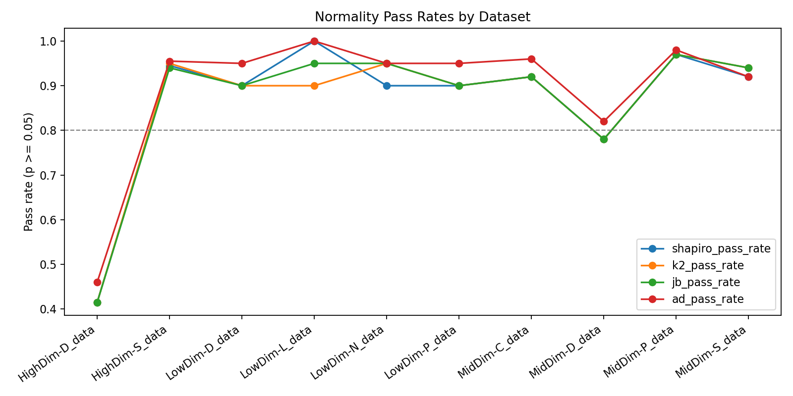
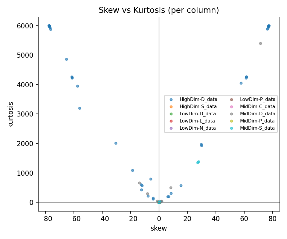
<p>The first two figures are useful as a dashboard view of the full benchmark:</p>

<ul>
  <li>the pass-rate plot summarises how often each dataset behaves in a Gaussian-like way across variables,</li>
  <li>the skew-versus-kurtosis plot shows whether the departures are driven more by asymmetry, tail-heaviness, or both.</li>
</ul>

<div class="diagnostics-figure-grid">
  <img src="/assets/normality-report/pass_rate_by_dataset.png" alt="Pass rates by dataset for four normality tests" />
  <img src="/assets/normality-report/skew_kurtosis_scatter.png" alt="Scatter plot of skewness versus kurtosis across datasets" />
</div>

<p>Already at this stage, two broad regimes appear:</p>

<ul>
  <li>datasets that are largely compatible with Gaussian assumptions,</li>
  <li>datasets with obvious tail or skew irregularities that should not be treated as clean linear-Gaussian baselines.</li>
</ul>

<h2 id="summary-table">Summary Table</h2>

<p>The table below aggregates the main diagnostics:</p>

<table>
  <thead>
    <tr>
      <th>Dataset</th>
      <th>n_cols</th>
      <th>Shapiro pass</th>
      <th>K2 pass</th>
      <th>JB pass</th>
      <th>AD pass</th>
      <th>mean</th>
      <th>skew</th>
      <th> </th>
      <th>mean</th>
      <th>kurt</th>
      <th> </th>
    </tr>
  </thead>
  <tbody>
    <tr>
      <td>HighDim-D_data</td>
      <td>200</td>
      <td>0.415</td>
      <td>0.415</td>
      <td>0.415</td>
      <td>0.460</td>
      <td>20.345</td>
      <td>1520.341</td>
      <td> </td>
      <td> </td>
      <td> </td>
      <td> </td>
    </tr>
    <tr>
      <td>HighDim-S_data</td>
      <td>200</td>
      <td>0.945</td>
      <td>0.950</td>
      <td>0.940</td>
      <td>0.955</td>
      <td>0.026</td>
      <td>0.047</td>
      <td> </td>
      <td> </td>
      <td> </td>
      <td> </td>
    </tr>
    <tr>
      <td>LowDim-D_data</td>
      <td>20</td>
      <td>0.900</td>
      <td>0.900</td>
      <td>0.900</td>
      <td>0.950</td>
      <td>0.053</td>
      <td>0.535</td>
      <td> </td>
      <td> </td>
      <td> </td>
      <td> </td>
    </tr>
    <tr>
      <td>LowDim-L_data</td>
      <td>20</td>
      <td>1.000</td>
      <td>0.900</td>
      <td>0.950</td>
      <td>1.000</td>
      <td>0.018</td>
      <td>0.063</td>
      <td> </td>
      <td> </td>
      <td> </td>
      <td> </td>
    </tr>
    <tr>
      <td>LowDim-N_data</td>
      <td>20</td>
      <td>0.900</td>
      <td>0.950</td>
      <td>0.950</td>
      <td>0.950</td>
      <td>0.024</td>
      <td>0.105</td>
      <td> </td>
      <td> </td>
      <td> </td>
      <td> </td>
    </tr>
    <tr>
      <td>LowDim-P_data</td>
      <td>20</td>
      <td>0.900</td>
      <td>0.900</td>
      <td>0.900</td>
      <td>0.950</td>
      <td>0.024</td>
      <td>0.047</td>
      <td> </td>
      <td> </td>
      <td> </td>
      <td> </td>
    </tr>
    <tr>
      <td>MidDim-C_data</td>
      <td>50</td>
      <td>0.920</td>
      <td>0.920</td>
      <td>0.920</td>
      <td>0.960</td>
      <td>0.029</td>
      <td>0.050</td>
      <td> </td>
      <td> </td>
      <td> </td>
      <td> </td>
    </tr>
    <tr>
      <td>MidDim-D_data</td>
      <td>100</td>
      <td>0.780</td>
      <td>0.780</td>
      <td>0.780</td>
      <td>0.820</td>
      <td>1.099</td>
      <td>70.508</td>
      <td> </td>
      <td> </td>
      <td> </td>
      <td> </td>
    </tr>
    <tr>
      <td>MidDim-P_data</td>
      <td>100</td>
      <td>0.970</td>
      <td>0.970</td>
      <td>0.970</td>
      <td>0.980</td>
      <td>0.024</td>
      <td>0.048</td>
      <td> </td>
      <td> </td>
      <td> </td>
      <td> </td>
    </tr>
    <tr>
      <td>MidDim-S_data</td>
      <td>100</td>
      <td>0.920</td>
      <td>0.940</td>
      <td>0.940</td>
      <td>0.920</td>
      <td>0.582</td>
      <td>27.523</td>
      <td> </td>
      <td> </td>
      <td> </td>
      <td> </td>
    </tr>
  </tbody>
</table>

<p>The stark contrast between datasets such as <strong>HighDim-S_data</strong> and <strong>HighDim-D_data</strong> makes the main point very clearly: not all synthetic benchmarks live in the same statistical world, even when they are being compared under the same causal-discovery umbrella.</p>

<h2 id="dataset-by-dataset-interpretation">Dataset-by-Dataset Interpretation</h2>

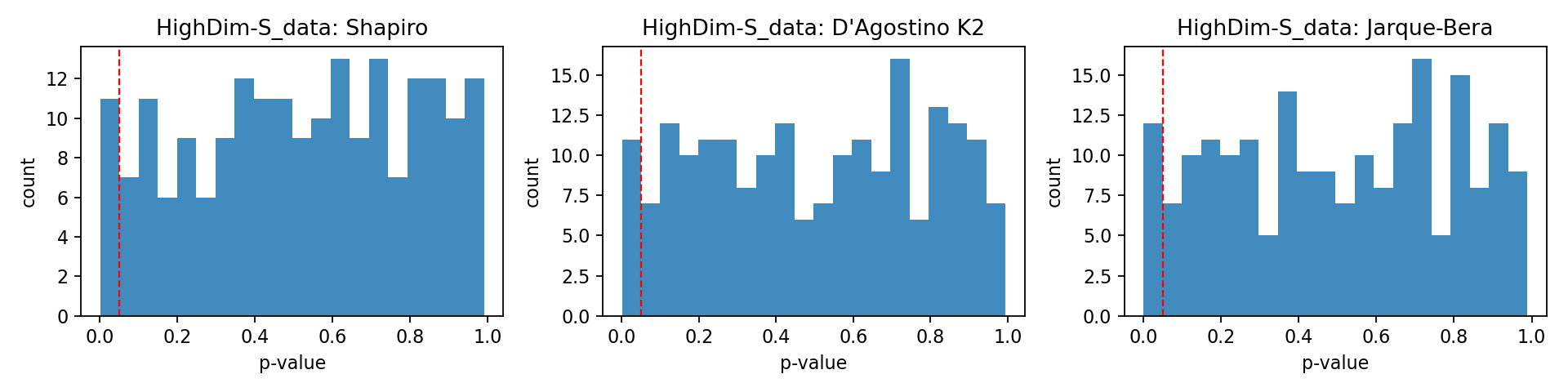
<h3 id="highdim-s_data-a-clean-gaussian-like-benchmark">HighDim-S_data: a clean Gaussian-like benchmark</h3>

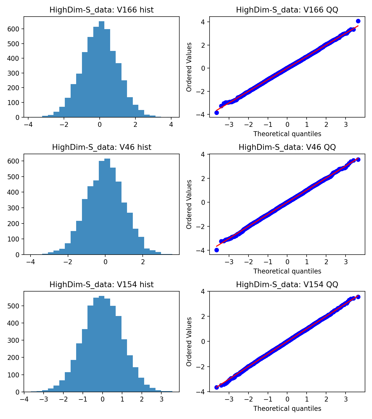
<p>This dataset behaves almost exactly as one would hope in a near-Gaussian regime:</p>

<ul>
  <li>pass rates are close to 0.95 across all four tests,</li>
  <li>mean absolute skewness is near zero,</li>
  <li>mean absolute kurtosis is also very low.</li>
</ul>

<p>That combination suggests a relatively well-behaved linear-Gaussian environment. In such a setting, <strong>PC</strong> and <strong>NOTEARS</strong> are natural reference methods because their structural assumptions are not being strongly violated from the start [1,6].</p>

<div class="diagnostics-figure-grid">
  <img src="/assets/normality-report/pvalues_HighDim-S_data.png" alt="Histogram of p-values for HighDim-S data" />
  <img src="/assets/normality-report/qq_hist_HighDim-S_data.png" alt="QQ plots and histograms for HighDim-S data" />
</div>

<h3 id="highdim-d_data-strong-evidence-of-non-gaussianity">HighDim-D_data: strong evidence of non-Gaussianity</h3>

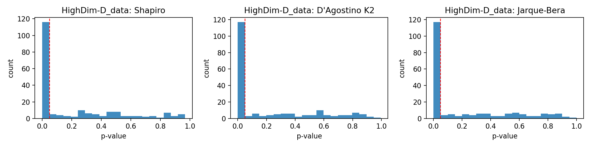
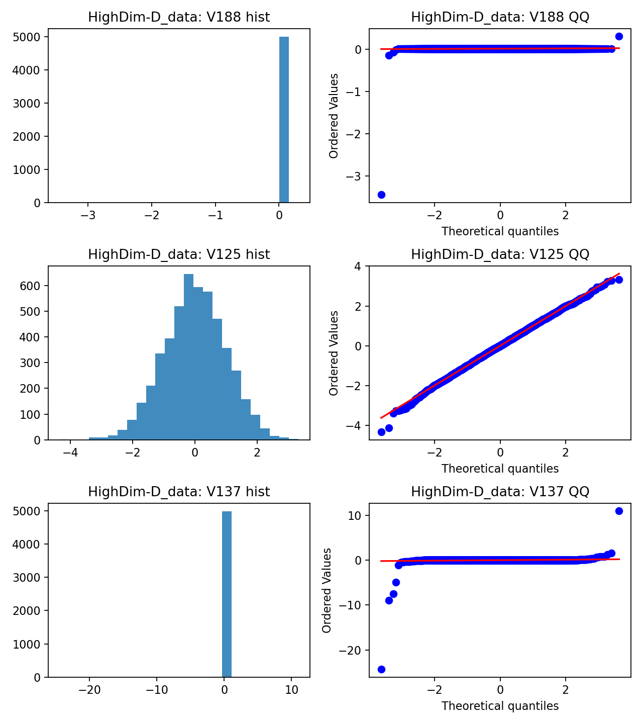
<p>This is the clearest non-Gaussian case in the benchmark:</p>

<ul>
  <li>pass rates are low across all tests,</li>
  <li>mean absolute skewness is extremely large,</li>
  <li>mean absolute kurtosis is extraordinarily large.</li>
</ul>

<p>This is not a mild deviation. It is a qualitatively different distributional regime. If one were to compare Gaussian-assumption methods against non-Gaussian methods here without acknowledging this structure, the comparison would be statistically misleading.</p>

<p>In this regime, <strong>LiNGAM</strong> becomes especially relevant because non-Gaussianity is part of the identifiability story rather than merely a nuisance [7]. If nonlinear mechanisms are also suspected, <strong>GraNDAG</strong> becomes a reasonable additional candidate [8].</p>

<div class="diagnostics-figure-grid">
  <img src="/assets/normality-report/pvalues_HighDim-D_data.png" alt="Histogram of p-values for HighDim-D data" />
  <img src="/assets/normality-report/qq_hist_HighDim-D_data.png" alt="QQ plots and histograms for HighDim-D data" />
</div>

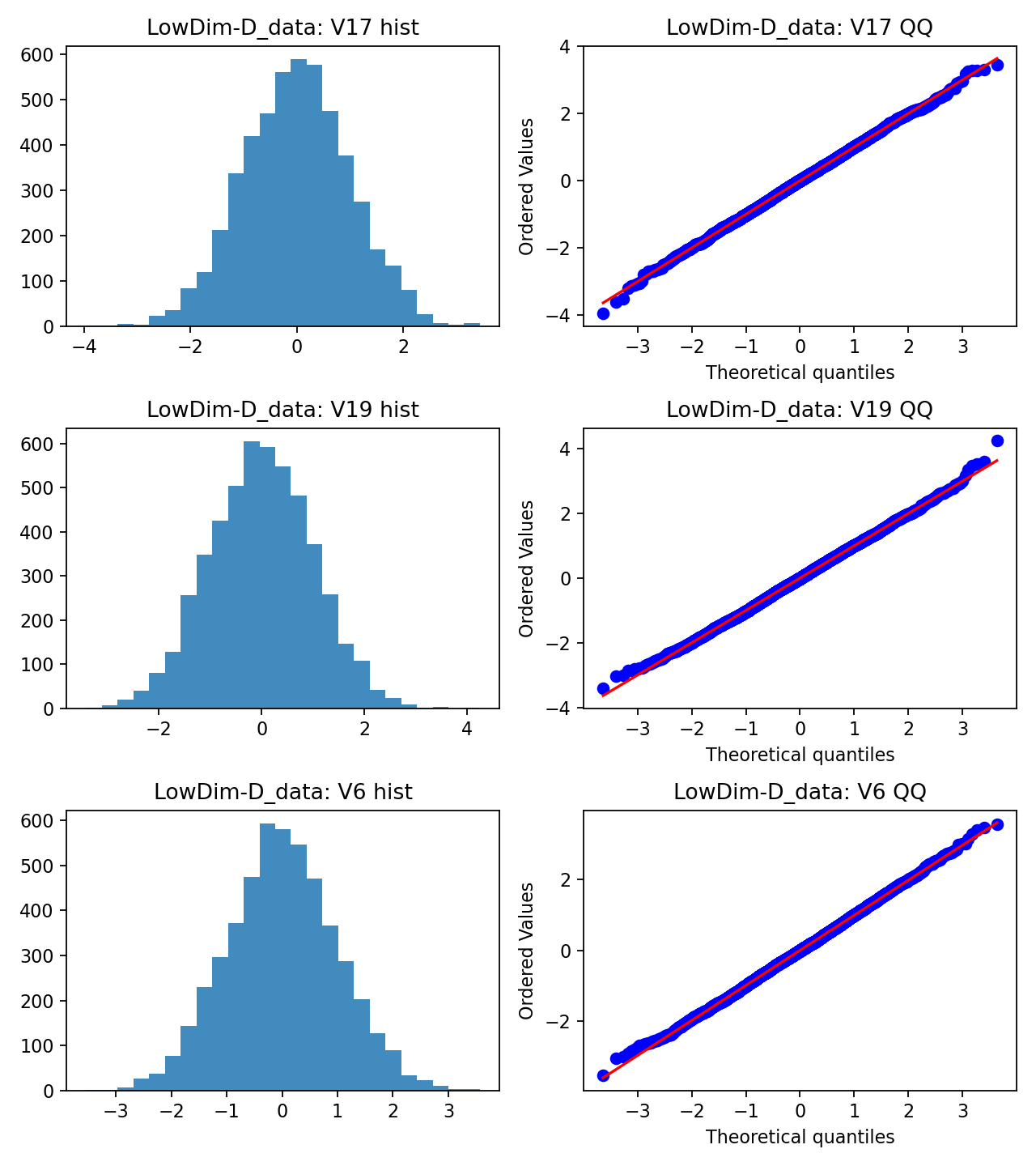
<h3 id="lowdim-datasets-mostly-well-behaved">LowDim datasets: mostly well-behaved</h3>

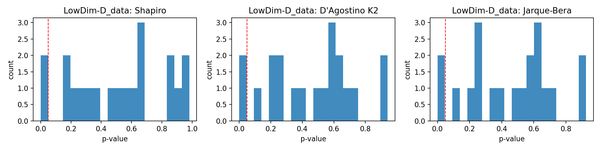
<p>The low-dimensional datasets are, for the most part, statistically calm:</p>

<ul>
  <li>pass rates are high,</li>
  <li>skewness is modest,</li>
  <li>kurtosis is small to moderate.</li>
</ul>

<p>LowDim-D_data shows somewhat more tail activity than the others, but not enough to move it into a clearly heavy-tailed regime. In practice, these look like sensible environments for <strong>PC</strong> and <strong>NOTEARS</strong>, with non-Gaussian methods serving more as robustness comparators than as necessary first choices.</p>

<div class="diagnostics-figure-grid">
  <img src="/assets/normality-report/pvalues_LowDim-D_data.png" alt="Histogram of p-values for LowDim-D data" />
  <img src="/assets/normality-report/qq_hist_LowDim-D_data.png" alt="QQ plots and histograms for LowDim-D data" />
</div>

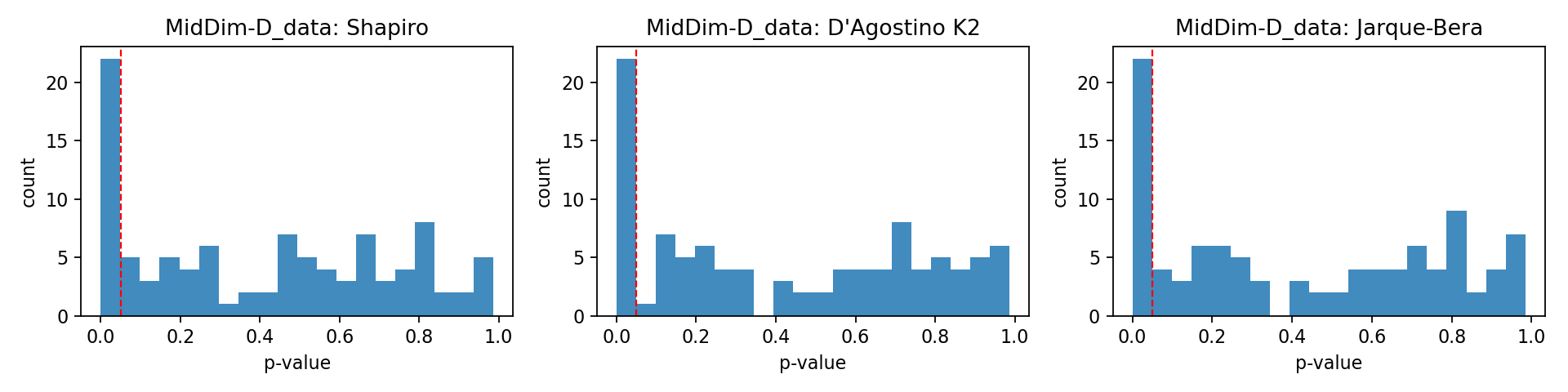
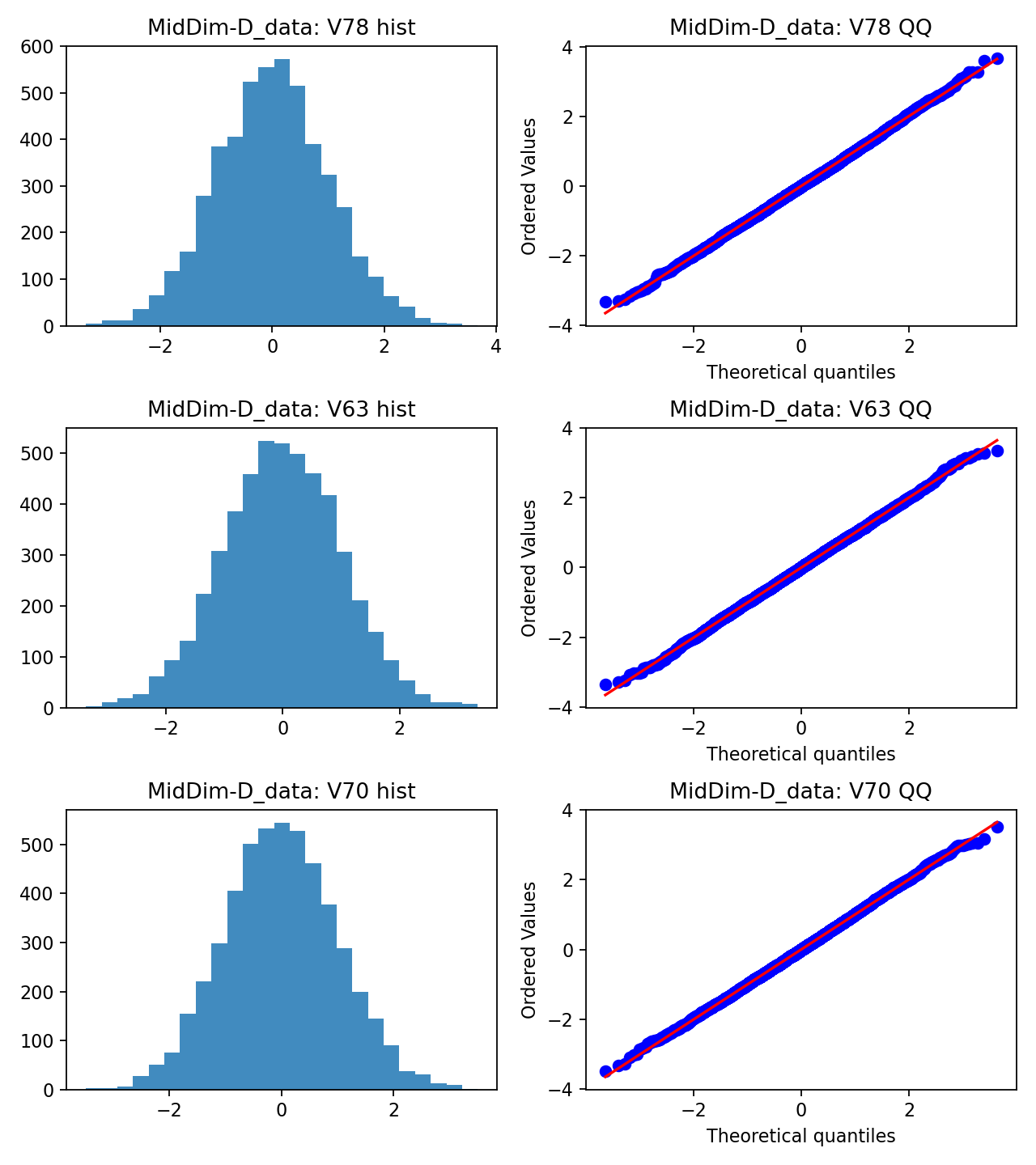
<h3 id="middim-d_data-tail-instability-becomes-visible">MidDim-D_data: tail instability becomes visible</h3>

<p>MidDim-D_data is more ambiguous than HighDim-D_data, but the signal is still clear:</p>

<ul>
  <li>pass rates drop to roughly 0.78-0.82,</li>
  <li>skewness and kurtosis are elevated,</li>
  <li>the distribution is not comfortably Gaussian.</li>
</ul>

<p>This is the kind of regime where a purely Gaussian interpretation becomes hard to defend, even if some variables still pass individual tests. I would therefore treat <strong>LiNGAM</strong> as a serious candidate here and keep <strong>GraNDAG</strong> in play if there is reason to expect nonlinear mechanisms.</p>

<div class="diagnostics-figure-grid">
  <img src="/assets/normality-report/pvalues_MidDim-D_data.png" alt="Histogram of p-values for MidDim-D data" />
  <img src="/assets/normality-report/qq_hist_MidDim-D_data.png" alt="QQ plots and histograms for MidDim-D data" />
</div>

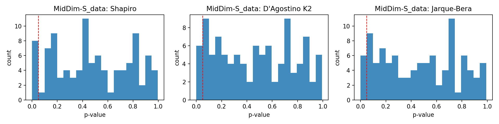
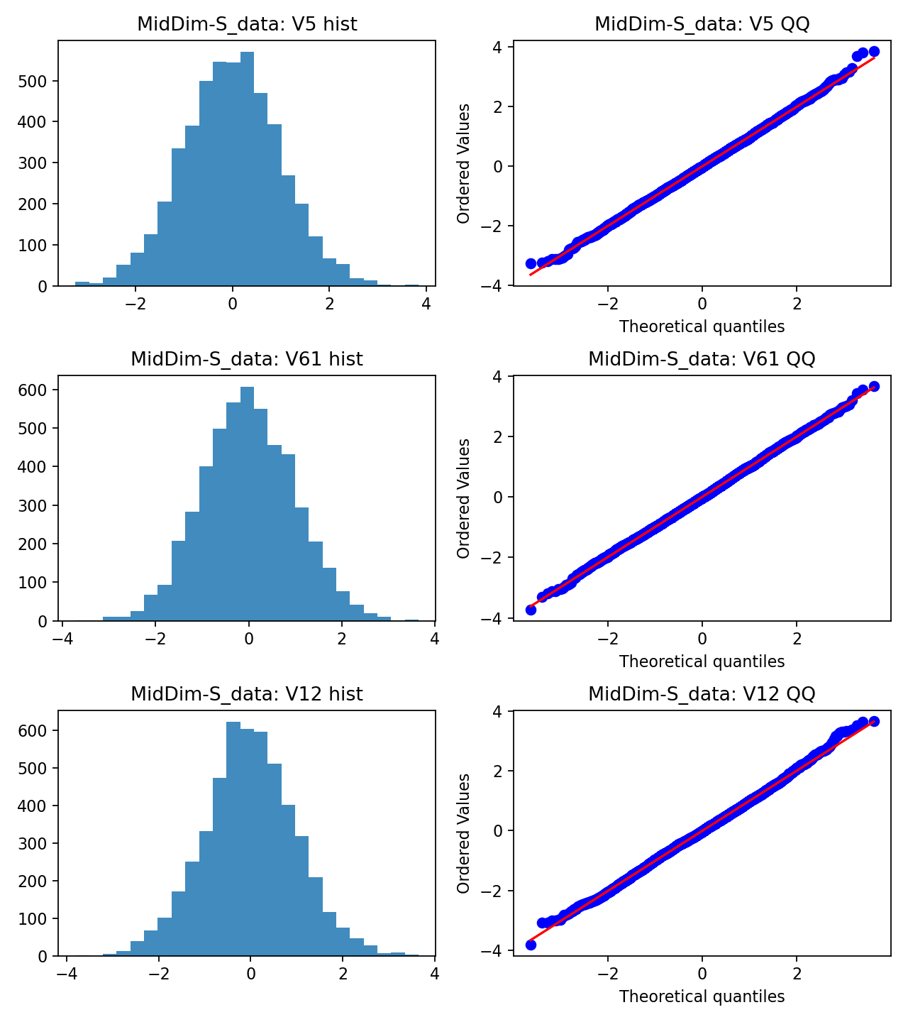
<h3 id="middim-s_data-mixed-structure">MidDim-S_data: mixed structure</h3>

<p>MidDim-S_data is the most interesting “borderline” case among the displayed examples:</p>

<ul>
  <li>pass rates remain fairly high,</li>
  <li>but mean kurtosis is still elevated,</li>
  <li>suggesting that many variables look acceptable while some carry heavier tails.</li>
</ul>

<p>This is precisely the type of dataset where relying on pass/fail counts alone can be misleading. A method that assumes global Gaussian comfort may still work reasonably well, but non-Gaussian structure is not absent.</p>

<p>That makes this a useful comparison regime:</p>

<ul>
  <li><strong>PC</strong> and <strong>NOTEARS</strong> remain defensible baselines,</li>
  <li><strong>LiNGAM</strong> may gain an advantage if the non-Gaussian subset is informative,</li>
  <li><strong>GraNDAG</strong> may be useful if there is also nonlinear mechanism complexity.</li>
</ul>

<div class="diagnostics-figure-grid">
  <img src="/assets/normality-report/pvalues_MidDim-S_data.png" alt="Histogram of p-values for MidDim-S data" />
  <img src="/assets/normality-report/qq_hist_MidDim-S_data.png" alt="QQ plots and histograms for MidDim-S data" />
</div>

<h2 id="a-practical-decision-framework">A Practical Decision Framework</h2>

<p>In applied work, I would summarise the diagnostic outcome in three broad regimes.</p>

<h3 id="regime-a-approximately-gaussian-low-skew-low-kurtosis">Regime A: approximately Gaussian, low skew, low kurtosis</h3>

<p>Typical signs:</p>

<ul>
  <li>high pass rates,</li>
  <li>QQ plots close to linear,</li>
  <li>skewness and kurtosis near zero.</li>
</ul>

<p>Recommended methods:</p>

<ul>
  <li><strong>PC</strong></li>
  <li><strong>NOTEARS</strong></li>
</ul>

<p>Optional:</p>

<ul>
  <li><strong>GraNDAG</strong> if there is substantive prior reason to expect nonlinear mechanisms.</li>
</ul>

<h3 id="regime-b-clearly-non-gaussian-or-heavy-tailed">Regime B: clearly non-Gaussian or heavy-tailed</h3>

<p>Typical signs:</p>

<ul>
  <li>low pass rates across several tests,</li>
  <li>heavy p-value mass near zero,</li>
  <li>strong skewness or tail-heaviness,</li>
  <li>visibly distorted QQ plots.</li>
</ul>

<p>Recommended methods:</p>

<ul>
  <li><strong>LiNGAM</strong></li>
</ul>

<p>Also reasonable:</p>

<ul>
  <li>robust comparisons using <strong>PC</strong> or <strong>NOTEARS</strong>, but with the explicit acknowledgment that the regime is unfavourable to clean Gaussian assumptions.</li>
</ul>

<h3 id="regime-c-mixed-or-structurally-ambiguous">Regime C: mixed or structurally ambiguous</h3>

<p>Typical signs:</p>

<ul>
  <li>moderate-to-high pass rates with some elevated kurtosis,</li>
  <li>acceptable marginals for many variables but a problematic subset,</li>
  <li>uncertainty about whether the main issue is non-Gaussianity, nonlinearity, or both.</li>
</ul>

<p>Recommended strategy:</p>

<ul>
  <li>compare <strong>PC</strong>, <strong>NOTEARS</strong>, <strong>LiNGAM</strong>, and <strong>GraNDAG</strong> in the same benchmark,</li>
  <li>interpret differences through diagnostics rather than only through final scores.</li>
</ul>

<h2 id="why-i-do-not-over-trust-p-values">Why I Do Not Over-Trust p-values</h2>

<p>This is worth stating explicitly.</p>

<p>In high-dimensional settings, we are effectively running one normality test per variable. That means:</p>

<ul>
  <li>some rejections occur by chance,</li>
  <li>very large sample sizes can make tests reject for very small and practically unimportant deviations,</li>
  <li>and a dataset can look mostly acceptable while still containing a few structurally important departures.</li>
</ul>

<p>That is why I treat p-values as one layer in the diagnostic stack, not as the entire story.</p>

<p>If the goal were formal multiple testing, one would need a correction strategy such as false-discovery-rate control [9]. Here, however, the aim is descriptive regime characterisation, not a definitive acceptance or rejection of Gaussianity as a universal property.</p>

<h2 id="limitations">Limitations</h2>

<p>These diagnostics are useful, but they are not complete.</p>

<p>Three limitations are especially important:</p>

<ol>
  <li>
    <p><strong>The tests are univariate.</strong><br />
A dataset can have Gaussian-looking marginals and still fail multivariate normality in a meaningful way.</p>
  </li>
  <li>
    <p><strong>Normal marginals do not imply causal simplicity.</strong><br />
Nonlinearity, heteroscedasticity, hidden confounding, or selection effects can still dominate the discovery problem.</p>
  </li>
  <li>
    <p><strong>Distributional diagnostics do not replace structural diagnostics.</strong><br />
They help us choose a better comparison framework, but they do not by themselves identify the correct graph.</p>
  </li>
</ol>

<h2 id="what-i-would-add-next">What I Would Add Next</h2>

<p>If I were extending this diagnostic pipeline, the next additions would be:</p>

<ul>
  <li>a multivariate normality diagnostic,</li>
  <li>a lightweight heteroscedasticity screen,</li>
  <li>a nonlinear dependence screen,</li>
  <li>and a stability summary linking distributional diagnostics to downstream graph-recovery performance.</li>
</ul>

<p>That would move the workflow from “distribution check” toward a more complete pre-analysis protocol for causal structure learning.</p>

<h2 id="final-takeaway">Final Takeaway</h2>

<p>The practical lesson is simple:</p>

<p><strong>Do not treat all synthetic causal-discovery benchmarks as though they represent the same statistical regime.</strong></p>

<p>Some are broadly Gaussian.<br />
Some are clearly heavy-tailed.<br />
Some are mixed.<br />
And that matters for identifiability, fairness of comparison, and interpretation of performance.</p>

<p>Running lightweight diagnostics before method comparison is therefore not cosmetic. It is part of doing the comparison responsibly.</p>

<h2 id="references">References</h2>

<ul>
  <li>[1] Spirtes, P., Glymour, C., &amp; Scheines, R. (2000). <em>Causation, Prediction, and Search</em> (2nd ed.). MIT Press.</li>
  <li>[2] Shapiro, S. S., &amp; Wilk, M. B. (1965). An analysis of variance test for normality (complete samples). <em>Biometrika</em>.</li>
  <li>[3] D’Agostino, R. (1973). Tests for departure from normality: empirical results for the distributions of $b_2$ and $\sqrt{b_1}$. <em>Biometrika</em>.</li>
  <li>[4] Jarque, C. M., &amp; Bera, A. K. (1980). Efficient tests for normality, homoscedasticity and serial independence of regression residuals. <em>Economics Letters</em>.</li>
  <li>[5] Anderson, T. W., &amp; Darling, D. A. (1954). A test of goodness of fit. <em>Journal of the American Statistical Association</em>.</li>
  <li>[6] Zheng, X., Aragam, B., Ravikumar, P., &amp; Xing, E. (2018). DAGs with NO TEARS: Continuous optimization for structure learning. <em>NeurIPS</em>.</li>
  <li>[7] Shimizu, S., Hoyer, P. O., Hyvarinen, A., &amp; Kerminen, A. (2006). A Linear Non-Gaussian Acyclic Model for Causal Discovery. <em>JMLR</em>.</li>
  <li>[8] Lachapelle, S., Brouillard, P., Deleu, T., &amp; Lacoste-Julien, S. (2019). Gradient-Based Neural DAG Learning. <em>ICLR</em>.</li>
  <li>[9] Benjamini, Y., &amp; Hochberg, Y. (1995). Controlling the false discovery rate: a practical and powerful approach to multiple testing. <em>JRSS-B</em>.</li>
</ul>]]></content><author><name>Inam Ullah Khan</name><email>i1n23@soton.ac.uk</email></author><category term="causal discovery" /><category term="normality" /><category term="statistics" /><category term="LiNGAM" /><category term="NOTEARS" /><category term="PC" /><category term="GraNDAG" /><summary type="html"><![CDATA[A professional diagnostic framework for checking Gaussianity, tail behaviour, and variable-wise distributional stability before comparing causal discovery methods.]]></summary></entry><entry><title type="html">Forbes Featured ‘The Eye as a Window to Systemic Health’</title><link href="https://inamullah-colab.github.io/news/2025/11/forbes-eye-window-systemic-health/" rel="alternate" type="text/html" title="Forbes Featured ‘The Eye as a Window to Systemic Health’" /><published>2025-11-05T12:00:00+00:00</published><updated>2025-11-05T12:00:00+00:00</updated><id>https://inamullah-colab.github.io/news/2025/11/forbes-eye-exams-whole-body-wellness</id><content type="html" xml:base="https://inamullah-colab.github.io/news/2025/11/forbes-eye-window-systemic-health/"><![CDATA[<p>Forbes published a feature on <strong>November 5, 2025</strong> titled
<a href="https://www.forbes.com/sites/williamhaseltine/2025/11/05/how-artificial-intelligence-makes-eye-exams-a-gateway-to-whole-body-wellness/">“How Artificial Intelligence Makes Eye Exams a Gateway to Whole-Body Wellness”</a>.</p>

<div class="euler-figure">
  <img src="/images/Systemic_Health.png" alt="Illustration connecting retinal imaging with systemic health" />
</div>

<p>The article features the broader idea at the center of our paper:
<strong>“The Eye as a Window to Systemic Health: A Survey of Retinal Imaging from Classical Techniques to Oculomics.”</strong></p>

<p>Its main message is that <strong>AI-enabled eye exams can act as a gateway to whole-body wellness</strong>. That framing closely matches the argument developed in our survey: retinal imaging is not limited to ocular assessment, but can reveal systemic cardiovascular, metabolic, and neurological signals through a non-invasive window into human health.</p>

<p>This coverage strengthens the broader clinical and translational relevance of oculomics and supports the view that retinal biomarkers, when combined with artificial intelligence, can contribute meaningfully to whole-body health assessment.</p>

<p>Related publication:
<a href="https://www.sciencedirect.com/science/article/pii/S305063282500023X">The Eye as a Window to Systemic Health: A Survey of Retinal Imaging from Classical Techniques to Oculomics</a></p>]]></content><author><name>Inam Ullah Khan</name><email>i1n23@soton.ac.uk</email></author><category term="news" /><category term="press" /><category term="forbes" /><category term="oculomics" /><category term="retinal-imaging" /><summary type="html"><![CDATA[Forbes featured the broader idea at the center of our paper 'The Eye as a Window to Systemic Health,' showing how AI-enabled eye exams can support whole-body wellness.]]></summary></entry><entry><title type="html">Euler Test</title><link href="https://inamullah-colab.github.io/euler-test/" rel="alternate" type="text/html" title="Euler Test" /><published>2024-04-18T12:00:00+00:00</published><updated>2024-04-18T12:00:00+00:00</updated><id>https://inamullah-colab.github.io/euler-test</id><content type="html" xml:base="https://inamullah-colab.github.io/euler-test/"><![CDATA[<h1 id="eulers-identity">Euler’s Identity</h1>

<p>This is a test post about Euler’s Identity.</p>

<p>The equation is: (e^{i\pi} + 1 = 0)</p>]]></content><author><name>Inam Ullah Khan</name><email>i1n23@soton.ac.uk</email></author><category term="mathematics" /><category term="euler" /><category term="test" /><summary type="html"><![CDATA[A simple test post about Euler's Identity]]></summary></entry><entry><title type="html">Five Constants, One Truth: Euler’s Identity</title><link href="https://inamullah-colab.github.io/posts/2024/04/five-constants-one-truth/" rel="alternate" type="text/html" title="Five Constants, One Truth: Euler’s Identity" /><published>2024-04-18T12:00:00+00:00</published><updated>2026-04-19T14:20:00+00:00</updated><id>https://inamullah-colab.github.io/posts/2024/04/five-constants-one-truth-eulers-identity</id><content type="html" xml:base="https://inamullah-colab.github.io/posts/2024/04/five-constants-one-truth/"><![CDATA[<h1 id="the-most-beautiful-equation-in-mathematics">The Most Beautiful Equation in Mathematics</h1>

<p>Euler’s identity is usually written as:</p>

\[e^{i\pi} + 1 = 0\]

<p>or equivalently:</p>

\[e^{i\pi} = -1\]

<p>This elegant equation unites five of the most important constants in all of mathematics:</p>

<ul>
  <li><code class="language-plaintext highlighter-rouge">0</code> as the additive identity</li>
  <li><code class="language-plaintext highlighter-rouge">1</code> as the multiplicative identity</li>
  <li><code class="language-plaintext highlighter-rouge">pi</code> as the circle constant</li>
  <li><code class="language-plaintext highlighter-rouge">e</code> as the growth constant</li>
  <li><code class="language-plaintext highlighter-rouge">i</code> as the imaginary unit</li>
</ul>

<p>Let’s visualize this relationship with a smaller moving diagram.</p>

<div class="euler-figure">
  <img src="/images/euler-waves-animated.svg" alt="Animated Euler diagram showing the unit circle together with the real cosine wave and the imaginary sine wave" />
</div>

<p>Euler’s identity elegantly connects five fundamental constants, each with its own profound significance.</p>

<h2 id="the-five-titans-of-mathematics">The Five Titans of Mathematics</h2>

<h3 id="0-the-additive-identity">0: The Additive Identity</h3>

<p>Zero represents nothingness, the empty baseline from which counting begins. It is the additive identity, because adding zero leaves a number unchanged. Without zero, the modern number system would be incomplete.</p>

<h3 id="1-the-multiplicative-identity">1: The Multiplicative Identity</h3>

<p>One is the foundation of counting and the multiplicative identity. Any number multiplied by one remains itself. It is the simplest positive integer and the basis from which the natural numbers are built.</p>

<h3 id="pi-the-circle-constant">pi: The Circle Constant</h3>

<p>$\pi \approx 3.14159\ldots$ emerges naturally from the geometry of circles and spheres. It is the ratio of a circle’s circumference to its diameter, appearing throughout physics, engineering, and natural phenomena. It is transcendental and irrational, so its decimal representation never repeats.</p>

<h3 id="e-the-growth-constant">e: The Growth Constant</h3>

<p>$e \approx 2.71828\ldots$ is the base of natural logarithms. It emerges from compound interest, exponential growth, and appears in physics, biology, and chemistry. When something grows at a rate proportional to its current size, $e$ appears naturally.</p>

<h3 id="i-the-imaginary-unit">i: The Imaginary Unit</h3>

<p>The imaginary unit satisfies:</p>

\[i^2 = -1\]

<p>While it seems abstract, complex numbers are essential for describing waves, quantum mechanics, electrical engineering, and signal processing. The label “imaginary” is historical. They are just as real as any other mathematical construct.</p>

<h2 id="the-profound-beauty">The Profound Beauty</h2>

<p>What makes Euler’s identity so remarkable is how five independent concepts, arising from completely different domains of mathematics, combine into one perfect equation:</p>

\[e^{i\pi} = -1\]

<p>This single equation encapsulates:</p>

<ul>
  <li>Exponential growth represented by <code class="language-plaintext highlighter-rouge">e</code></li>
  <li>Complex rotation represented by <code class="language-plaintext highlighter-rouge">i</code></li>
  <li>The perfect angle represented by <code class="language-plaintext highlighter-rouge">pi</code>, which equals exactly half a circle</li>
  <li>Perfect opposition through <code class="language-plaintext highlighter-rouge">-1</code></li>
  <li>Complete harmony through <code class="language-plaintext highlighter-rouge">e^(i pi) + 1 = 0</code></li>
</ul>

<p>The beauty is not just mathematical elegance. It is a revelation that these seemingly disparate concepts are deeply interconnected. They are not separate truths. They are facets of a single underlying reality.</p>

<h2 id="the-engine-and-steering-wheel-analogy">The Engine and Steering Wheel Analogy</h2>

<p>Think of Euler’s identity like a car journey:</p>

<ul>
  <li><code class="language-plaintext highlighter-rouge">e</code> is the engine. It provides the continuous power and growth.</li>
  <li><code class="language-plaintext highlighter-rouge">i</code> is the steering wheel. It controls the direction, allowing rotation in the complex plane.</li>
  <li><code class="language-plaintext highlighter-rouge">pi</code> is the perfect turn, exactly half a circle or 180 degrees.</li>
  <li>The result <code class="language-plaintext highlighter-rouge">-1</code> means you arrive exactly opposite your starting point</li>
</ul>

<p>The equation <code class="language-plaintext highlighter-rouge">e^(i pi) + 1 = 0</code> is like saying: if you drive with the engine running while turning the steering wheel exactly halfway around, then add your starting position to your ending position, you get perfect balance, zero.</p>

<div class="euler-figure">
  <img src="/images/euler-engine-steering-animated.svg" alt="Animated engine and steering wheel analogy for Euler's identity" />
</div>

<h2 id="the-engineering-and-physics-interpretation">The Engineering and Physics Interpretation</h2>

<p>Imagine standing at point <code class="language-plaintext highlighter-rouge">+1</code> on the real number line and applying the transformation <code class="language-plaintext highlighter-rouge">e^(i pi)</code>:</p>

<ul>
  <li>The exponent <code class="language-plaintext highlighter-rouge">i pi</code> instructs the exponential to perform a complex rotation of <code class="language-plaintext highlighter-rouge">pi</code> radians in the complex plane</li>
  <li>Starting from position <code class="language-plaintext highlighter-rouge">+1</code>, a <code class="language-plaintext highlighter-rouge">pi</code> radian rotation brings you exactly to <code class="language-plaintext highlighter-rouge">-1</code></li>
  <li>The exponential function maintains the magnitude at exactly <code class="language-plaintext highlighter-rouge">1</code></li>
  <li>The result is a perfect 180-degree reversal without any change in length</li>
</ul>

<p>So the transformation gives <code class="language-plaintext highlighter-rouge">e^(i pi) = -1</code>, and therefore:</p>

\[e^{i\pi} + 1 = 0\]

<p>In physics, this describes how oscillating systems behave. Waves naturally follow the pattern <code class="language-plaintext highlighter-rouge">e^(i omega t)</code>, combining an exponential envelope, oscillation frequency, and phase relationships. This is how alternating current circuits operate, how radio waves propagate, and how quantum wavefunctions evolve through time.</p>

<p>Euler’s identity is fundamental to describing periodic and oscillating phenomena:</p>

<ul>
  <li>Quantum mechanics uses complex exponentials of the form <code class="language-plaintext highlighter-rouge">e^(i theta)</code> to describe probability waves and superposition</li>
  <li>Wave physics describes sound, light, and water waves using <code class="language-plaintext highlighter-rouge">e^(i omega t)</code></li>
  <li>Control systems use <code class="language-plaintext highlighter-rouge">e^(i theta)</code> to design stable feedback loops</li>
  <li>Electromagnetism is elegantly expressed using complex-number methods</li>
  <li>Signal processing relies on Fourier transforms, which decompose signals into <code class="language-plaintext highlighter-rouge">e^(i omega t)</code> components</li>
</ul>

<h2 id="why-this-matters-applications-across-science-and-technology">Why This Matters: Applications Across Science and Technology</h2>

<h3 id="physics-and-engineering">Physics and Engineering</h3>

<p>These ideas are not decorative. They are the working language of waves, fields, and oscillatory systems.</p>

<h3 id="statistics-and-data-science">Statistics and Data Science</h3>

<p>Though less obvious, Euler’s identity also underlies modern data analysis.</p>

<div class="euler-formula-card">
Fourier analysis of time-series data uses the kernel

$$e^{-2\pi i k n / N}$$

to identify periodic patterns.
</div>

<div class="euler-formula-card">
Characteristic functions in probability take the form

$$\mathbb{E}[e^{itX}]$$

which connects random variables to Fourier analysis.
</div>

<div class="euler-formula-card">
Circular statistics uses

$$e^{i\theta}$$

for angles, phases, and cyclic effects.
</div>

<div class="euler-formula-card">
Eigendecomposition methods connect naturally to complex-valued analysis, and Bayesian computational methods often work in spaces where complex exponentials remain fundamental.
</div>

<h3 id="computer-science-and-artificial-intelligence">Computer Science and Artificial Intelligence</h3>

<p>Euler’s identity is surprisingly central to modern AI and computing:</p>

<ul>
  <li>Fourier-based methods are used in machine learning and scientific computing</li>
  <li>Neural networks that use Fourier features rely on sine and cosine structure derived from complex exponentials</li>
  <li>Audio processing and speech recognition rely on Fourier decompositions</li>
  <li>Image compression methods are derived from related harmonic ideas</li>
  <li>Computer vision models sometimes encode rotational structure using harmonic features</li>
  <li>Quantum computing represents operations with unitary matrices involving complex exponentials</li>
  <li>Equivariant and symmetry-aware neural networks use the same mathematical foundations</li>
  <li>Optimization in some complex-valued learning systems uses <code class="language-plaintext highlighter-rouge">z = e^(i theta)</code> style parameterizations</li>
</ul>

<h3 id="real-world-ai-applications">Real-World AI Applications</h3>

<p>These ideas show up in practical systems:</p>

<ul>
  <li>speech recognition</li>
  <li>music generation</li>
  <li>recommendation systems that analyze periodic patterns</li>
  <li>time-series forecasting</li>
  <li>image and vision pipelines operating in the frequency domain</li>
</ul>

<h2 id="the-deeper-significance">The Deeper Significance</h2>

<p>What makes Euler’s identity special is that it connects:</p>

<ol>
  <li>Pure mathematics</li>
  <li>Physical reality</li>
  <li>Information and signal theory</li>
  <li>Modern technology</li>
</ol>

<p>All of that appears through one elegantly compact equation.</p>

<p>This suggests that Euler’s identity is not just a mathematical curiosity. It is a compact description of how reality encodes and transmits information across scales, from quantum mechanics to classical physics to artificial intelligence systems.</p>

<p>In many ways, understanding Euler’s identity is understanding part of the language that nature uses to communicate with itself. Its beauty lies not just in mathematical correctness, but in revealing that seemingly separate mathematical concepts are fundamentally connected.</p>]]></content><author><name>Inam Ullah Khan</name><email>i1n23@soton.ac.uk</email></author><category term="mathematics" /><category term="euler" /><category term="identity" /><category term="complex numbers" /><category term="physics" /><category term="ai" /><summary type="html"><![CDATA[A cleaned web version of the PDF article on how Euler's identity connects 0, 1, pi, e, and i across mathematics, physics, and computing.]]></summary></entry></feed>