
Normality and Variance Diagnostics for Causal Discovery
Published:
Normality and Variance Diagnostics for Causal Discovery
Before comparing causal discovery methods, I usually ask a simpler question first:
What kind of data regime am I actually dealing with?
That question matters more than it may seem. Many causal discovery methods do not fail because the optimisation was poor or because the code was wrong. They fail because the data violate the assumptions under which the method is identifiable, stable, or interpretable.
This post describes a practical diagnostic framework I use before model comparison. The goal is not to “prove” that a dataset is Gaussian or non-Gaussian in some absolute sense. The goal is more operational:
- identify whether the marginals are broadly Gaussian-like,
- detect heavy tails or skewness early,
- understand how much heterogeneity is present across variables,
- and use that information to choose a more defensible set of baseline methods.
The examples here come from synthetic benchmark datasets, but the same logic applies more broadly when preparing a causal discovery workflow.
Why These Diagnostics Matter
Causal discovery is not one method. It is a family of methods built on different structural assumptions:
- linear versus nonlinear functional relations,
- Gaussian versus non-Gaussian disturbances,
- smooth versus heavy-tailed distributions,
- stable versus unstable scale behaviour,
- low-dimensional versus high-dimensional regimes.
Those distinctions are not cosmetic. They directly influence whether a method is merely computationally applicable or actually statistically appropriate.
For example:
- PC is often natural in approximately Gaussian settings when conditional independence structure is informative.
- NOTEARS is strong when the data are reasonably well described by a linear structural model and continuous optimisation is a sensible route for graph recovery.
- LiNGAM becomes especially relevant when non-Gaussianity is not just noise but a source of identifiability.
- GraNDAG is more attractive when one expects nonlinear mechanisms and wants a DAG-learning procedure that is not restricted to a linear-Gaussian world.
That is why I prefer to begin with diagnostics rather than immediately launching into performance tables.
Reproducibility
The script used to compute the summaries and plots is included in the repository:
assets/normality-report/normality_tests.py
To run it locally:
python assets/normality-report/normality_tests.py
Benchmark Datasets
The diagnostic suite was run on synthetic datasets of different dimensionalities. Each dataset contains 6,000 rows, with the number of variables varying by benchmark setting:
| Dataset | Shape (rows x columns) |
|---|---|
| LowDim-D_data | 6000 x 20 |
| LowDim-L_data | 6000 x 20 |
| LowDim-N_data | 6000 x 20 |
| LowDim-P_data | 6000 x 20 |
| MidDim-C_data | 6000 x 50 |
| MidDim-D_data | 6000 x 100 |
| MidDim-P_data | 6000 x 100 |
| MidDim-S_data | 6000 x 100 |
| HighDim-D_data | 6000 x 200 |
| HighDim-S_data | 6000 x 200 |
The point of keeping these datasets together in one diagnostic view is not merely convenience. It allows us to reason about whether the distributional structure shifts with dimensionality, and whether the “difficulty” of a benchmark is only graph-theoretic or also distributional.
What Is Actually Being Tested?
A normality test does not answer the philosophical question “Is this variable normal?” It answers a narrower statistical question:
Does the observed sample look inconsistent with a Gaussian distribution under the sensitivity profile of this test?
Different tests detect different types of departure:
- Shapiro-Wilk is widely used and often strong for common deviations from normality, especially in standard applied settings [2].
- D’Agostino K-squared combines skewness and kurtosis into one omnibus test and is particularly convenient in moderate-to-large sample settings [3].
- Jarque-Bera is another skewness-kurtosis-based omnibus diagnostic [4].
- Anderson-Darling tends to be more sensitive in the tails, which is valuable when heavy-tailed behaviour matters [5].
This is why I do not interpret a single p-value in isolation. I read the tests jointly, alongside:
- skewness,
- kurtosis,
- p-value histograms,
- QQ plots,
- and cross-dataset pass-rate summaries.
A Practical Reading Strategy
When reading this kind of report, I use a layered approach.
1. Start with pass rates
Pass rates give a quick view of how many variables remain consistent with Gaussianity at the chosen threshold. They are not a proof of normality, but they are useful as a regime summary.
2. Look at skewness and kurtosis
A variable can pass some normality tests and still show meaningful tail behaviour. That is why skewness and kurtosis are important complementary summaries.
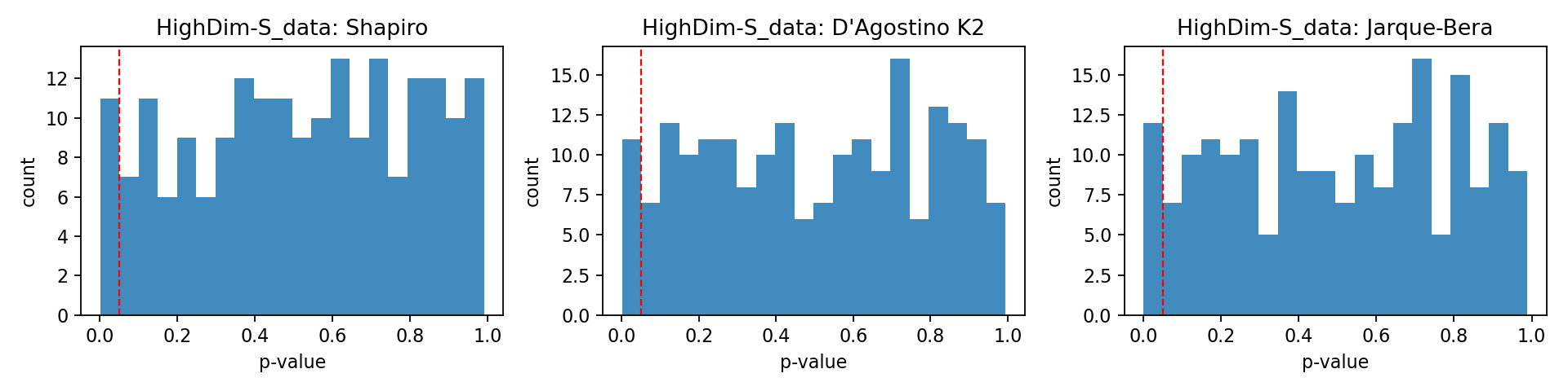
3. Inspect p-value histograms
If p-values pile up near zero, that usually indicates systematic deviation rather than isolated rejections.
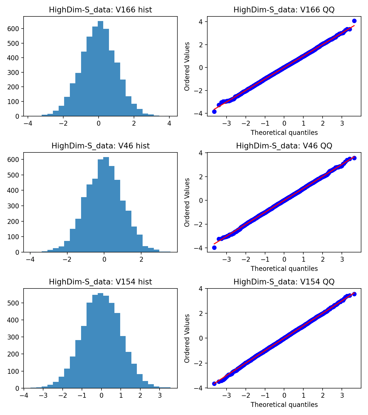
4. Inspect QQ plots
QQ plots often show the nature of the departure more clearly than a test statistic does:
- curvature suggests skewness,
- tail separation suggests heavy tails,
- broad instability suggests heterogeneous variable behaviour.
Overview Figures
The first two figures are useful as a dashboard view of the full benchmark:
- the pass-rate plot summarises how often each dataset behaves in a Gaussian-like way across variables,
- the skew-versus-kurtosis plot shows whether the departures are driven more by asymmetry, tail-heaviness, or both.
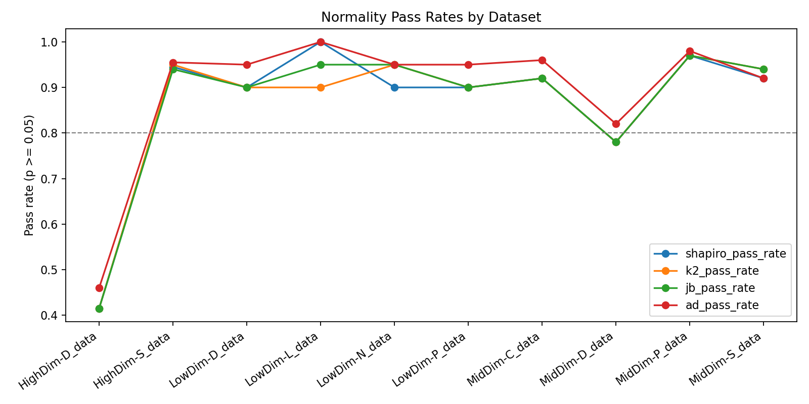
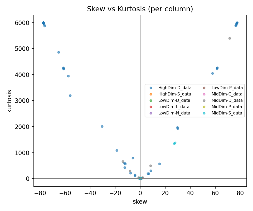
Already at this stage, two broad regimes appear:
- datasets that are largely compatible with Gaussian assumptions,
- datasets with obvious tail or skew irregularities that should not be treated as clean linear-Gaussian baselines.
Summary Table
The table below aggregates the main diagnostics:
| Dataset | n_cols | Shapiro pass | K2 pass | JB pass | AD pass | mean | skew | mean | kurt | ||
|---|---|---|---|---|---|---|---|---|---|---|---|
| HighDim-D_data | 200 | 0.415 | 0.415 | 0.415 | 0.460 | 20.345 | 1520.341 | ||||
| HighDim-S_data | 200 | 0.945 | 0.950 | 0.940 | 0.955 | 0.026 | 0.047 | ||||
| LowDim-D_data | 20 | 0.900 | 0.900 | 0.900 | 0.950 | 0.053 | 0.535 | ||||
| LowDim-L_data | 20 | 1.000 | 0.900 | 0.950 | 1.000 | 0.018 | 0.063 | ||||
| LowDim-N_data | 20 | 0.900 | 0.950 | 0.950 | 0.950 | 0.024 | 0.105 | ||||
| LowDim-P_data | 20 | 0.900 | 0.900 | 0.900 | 0.950 | 0.024 | 0.047 | ||||
| MidDim-C_data | 50 | 0.920 | 0.920 | 0.920 | 0.960 | 0.029 | 0.050 | ||||
| MidDim-D_data | 100 | 0.780 | 0.780 | 0.780 | 0.820 | 1.099 | 70.508 | ||||
| MidDim-P_data | 100 | 0.970 | 0.970 | 0.970 | 0.980 | 0.024 | 0.048 | ||||
| MidDim-S_data | 100 | 0.920 | 0.940 | 0.940 | 0.920 | 0.582 | 27.523 |
The stark contrast between datasets such as HighDim-S_data and HighDim-D_data makes the main point very clearly: not all synthetic benchmarks live in the same statistical world, even when they are being compared under the same causal-discovery umbrella.
Dataset-by-Dataset Interpretation
HighDim-S_data: a clean Gaussian-like benchmark
This dataset behaves almost exactly as one would hope in a near-Gaussian regime:
- pass rates are close to 0.95 across all four tests,
- mean absolute skewness is near zero,
- mean absolute kurtosis is also very low.
That combination suggests a relatively well-behaved linear-Gaussian environment. In such a setting, PC and NOTEARS are natural reference methods because their structural assumptions are not being strongly violated from the start [1,6].
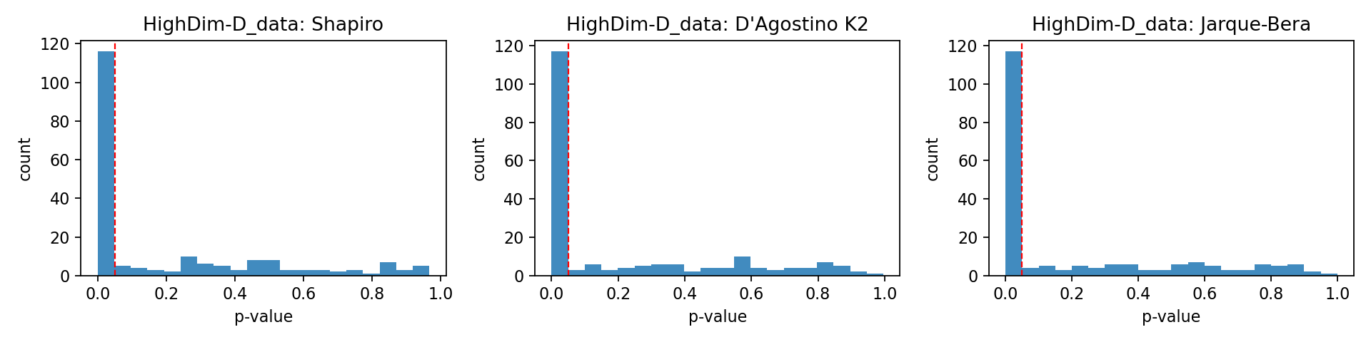
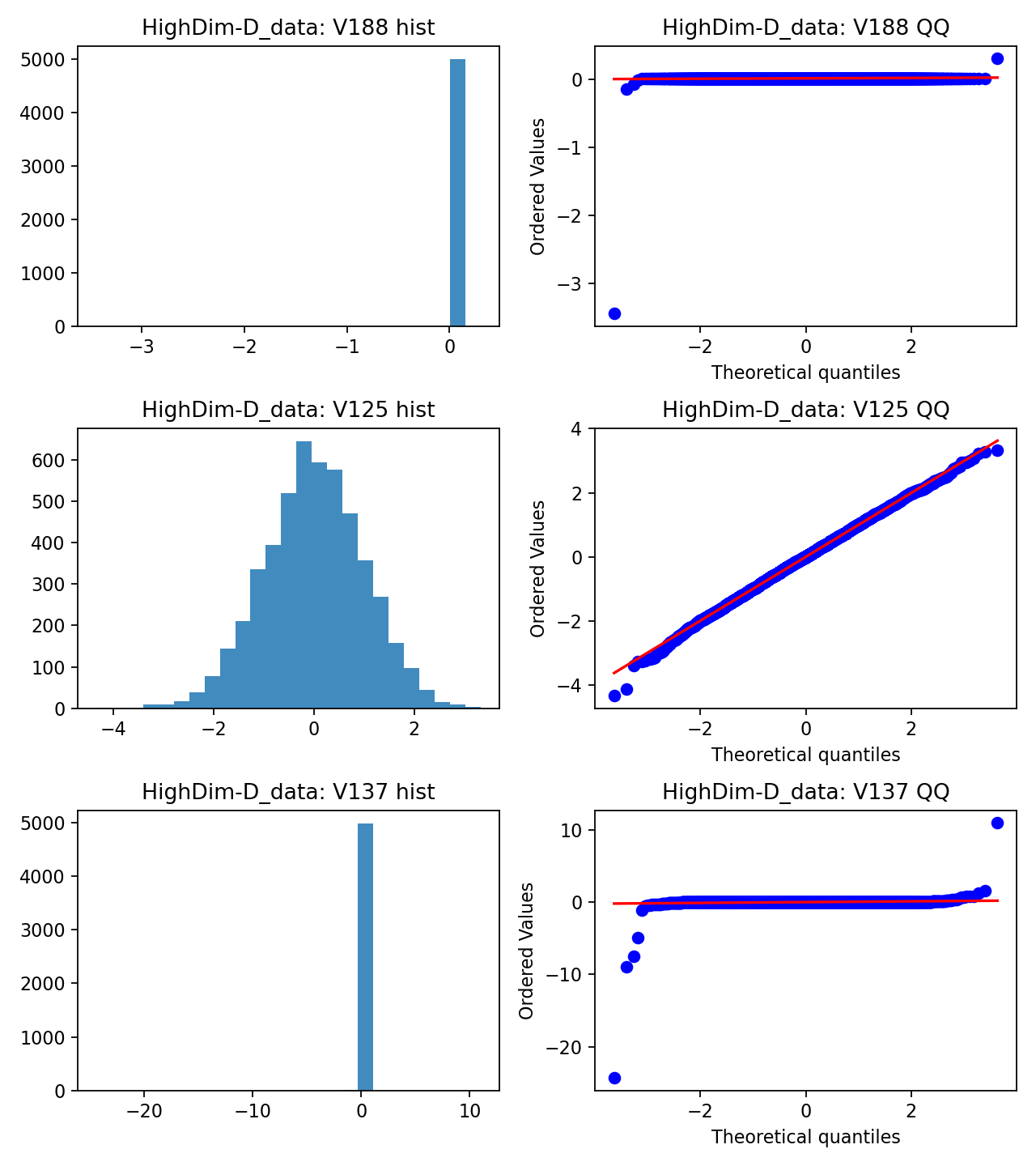
HighDim-D_data: strong evidence of non-Gaussianity
This is the clearest non-Gaussian case in the benchmark:
- pass rates are low across all tests,
- mean absolute skewness is extremely large,
- mean absolute kurtosis is extraordinarily large.
This is not a mild deviation. It is a qualitatively different distributional regime. If one were to compare Gaussian-assumption methods against non-Gaussian methods here without acknowledging this structure, the comparison would be statistically misleading.
In this regime, LiNGAM becomes especially relevant because non-Gaussianity is part of the identifiability story rather than merely a nuisance [7]. If nonlinear mechanisms are also suspected, GraNDAG becomes a reasonable additional candidate [8].
LowDim datasets: mostly well-behaved
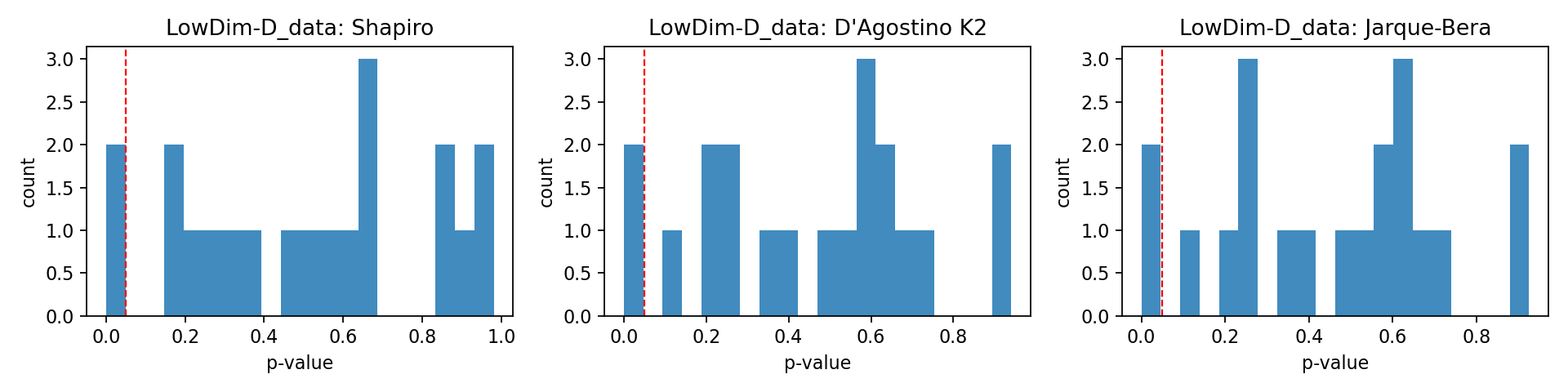
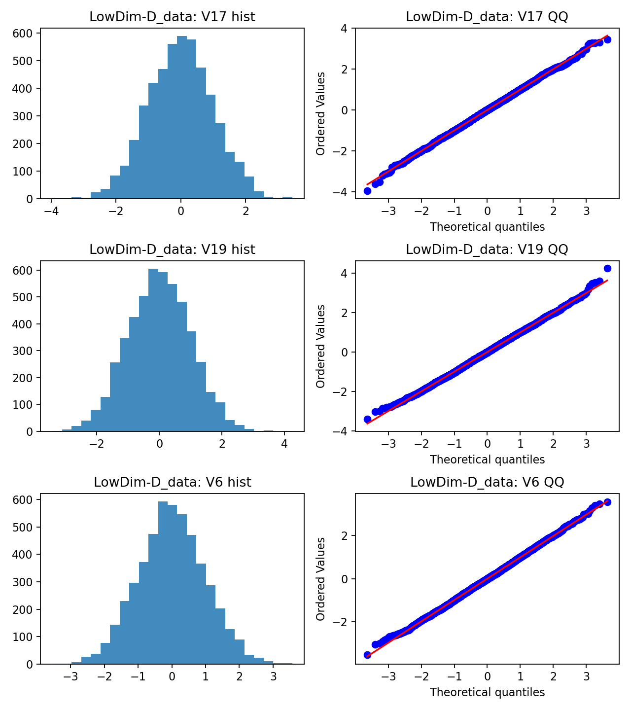
The low-dimensional datasets are, for the most part, statistically calm:
- pass rates are high,
- skewness is modest,
- kurtosis is small to moderate.
LowDim-D_data shows somewhat more tail activity than the others, but not enough to move it into a clearly heavy-tailed regime. In practice, these look like sensible environments for PC and NOTEARS, with non-Gaussian methods serving more as robustness comparators than as necessary first choices.
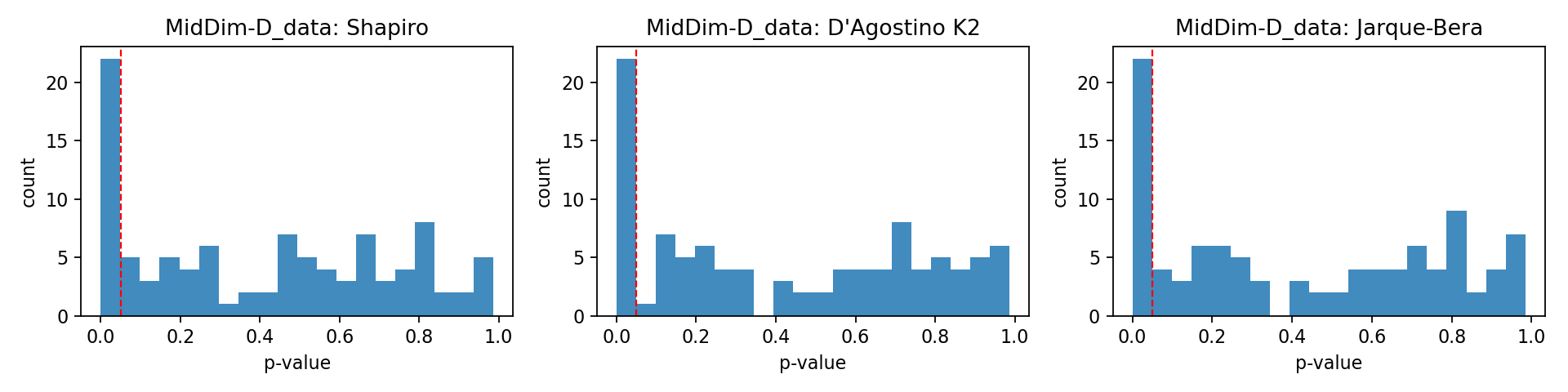
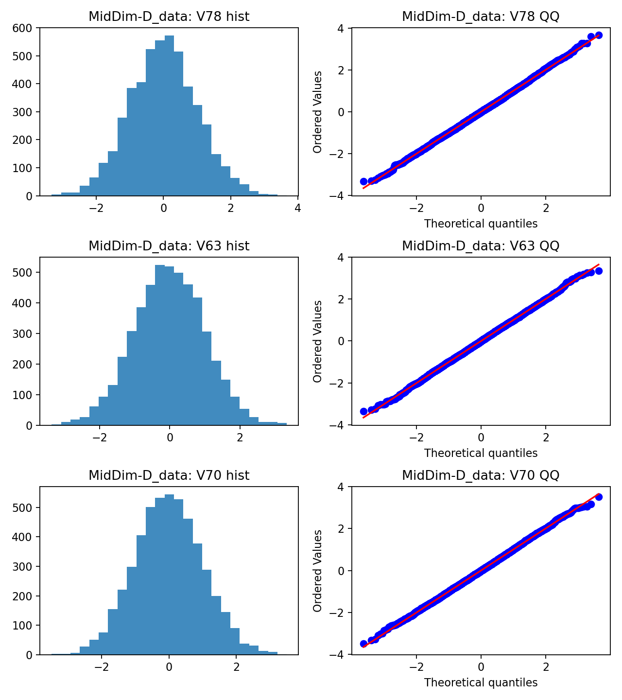
MidDim-D_data: tail instability becomes visible
MidDim-D_data is more ambiguous than HighDim-D_data, but the signal is still clear:
- pass rates drop to roughly 0.78-0.82,
- skewness and kurtosis are elevated,
- the distribution is not comfortably Gaussian.
This is the kind of regime where a purely Gaussian interpretation becomes hard to defend, even if some variables still pass individual tests. I would therefore treat LiNGAM as a serious candidate here and keep GraNDAG in play if there is reason to expect nonlinear mechanisms.
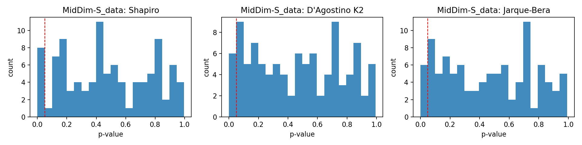
MidDim-S_data: mixed structure
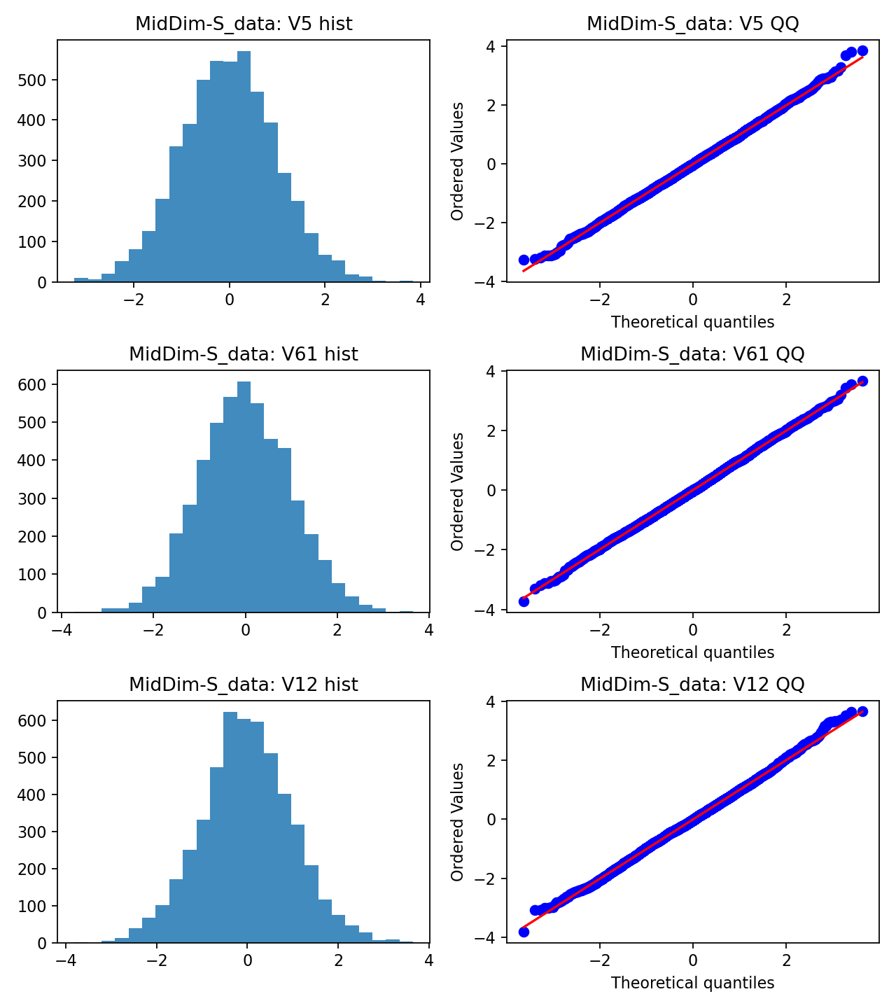
MidDim-S_data is the most interesting “borderline” case among the displayed examples:
- pass rates remain fairly high,
- but mean kurtosis is still elevated,
- suggesting that many variables look acceptable while some carry heavier tails.
This is precisely the type of dataset where relying on pass/fail counts alone can be misleading. A method that assumes global Gaussian comfort may still work reasonably well, but non-Gaussian structure is not absent.
That makes this a useful comparison regime:
- PC and NOTEARS remain defensible baselines,
- LiNGAM may gain an advantage if the non-Gaussian subset is informative,
- GraNDAG may be useful if there is also nonlinear mechanism complexity.
A Practical Decision Framework
In applied work, I would summarise the diagnostic outcome in three broad regimes.
Regime A: approximately Gaussian, low skew, low kurtosis
Typical signs:
- high pass rates,
- QQ plots close to linear,
- skewness and kurtosis near zero.
Recommended methods:
- PC
- NOTEARS
Optional:
- GraNDAG if there is substantive prior reason to expect nonlinear mechanisms.
Regime B: clearly non-Gaussian or heavy-tailed
Typical signs:
- low pass rates across several tests,
- heavy p-value mass near zero,
- strong skewness or tail-heaviness,
- visibly distorted QQ plots.
Recommended methods:
- LiNGAM
Also reasonable:
- robust comparisons using PC or NOTEARS, but with the explicit acknowledgment that the regime is unfavourable to clean Gaussian assumptions.
Regime C: mixed or structurally ambiguous
Typical signs:
- moderate-to-high pass rates with some elevated kurtosis,
- acceptable marginals for many variables but a problematic subset,
- uncertainty about whether the main issue is non-Gaussianity, nonlinearity, or both.
Recommended strategy:
- compare PC, NOTEARS, LiNGAM, and GraNDAG in the same benchmark,
- interpret differences through diagnostics rather than only through final scores.
Why I Do Not Over-Trust p-values
This is worth stating explicitly.
In high-dimensional settings, we are effectively running one normality test per variable. That means:
- some rejections occur by chance,
- very large sample sizes can make tests reject for very small and practically unimportant deviations,
- and a dataset can look mostly acceptable while still containing a few structurally important departures.
That is why I treat p-values as one layer in the diagnostic stack, not as the entire story.
If the goal were formal multiple testing, one would need a correction strategy such as false-discovery-rate control [9]. Here, however, the aim is descriptive regime characterisation, not a definitive acceptance or rejection of Gaussianity as a universal property.
Limitations
These diagnostics are useful, but they are not complete.
Three limitations are especially important:
The tests are univariate.
A dataset can have Gaussian-looking marginals and still fail multivariate normality in a meaningful way.Normal marginals do not imply causal simplicity.
Nonlinearity, heteroscedasticity, hidden confounding, or selection effects can still dominate the discovery problem.Distributional diagnostics do not replace structural diagnostics.
They help us choose a better comparison framework, but they do not by themselves identify the correct graph.
What I Would Add Next
If I were extending this diagnostic pipeline, the next additions would be:
- a multivariate normality diagnostic,
- a lightweight heteroscedasticity screen,
- a nonlinear dependence screen,
- and a stability summary linking distributional diagnostics to downstream graph-recovery performance.
That would move the workflow from “distribution check” toward a more complete pre-analysis protocol for causal structure learning.
Final Takeaway
The practical lesson is simple:
Do not treat all synthetic causal-discovery benchmarks as though they represent the same statistical regime.
Some are broadly Gaussian.
Some are clearly heavy-tailed.
Some are mixed.
And that matters for identifiability, fairness of comparison, and interpretation of performance.
Running lightweight diagnostics before method comparison is therefore not cosmetic. It is part of doing the comparison responsibly.
References
- [1] Spirtes, P., Glymour, C., & Scheines, R. (2000). Causation, Prediction, and Search (2nd ed.). MIT Press.
- [2] Shapiro, S. S., & Wilk, M. B. (1965). An analysis of variance test for normality (complete samples). Biometrika.
- [3] D’Agostino, R. (1973). Tests for departure from normality: empirical results for the distributions of $b_2$ and $\sqrt{b_1}$. Biometrika.
- [4] Jarque, C. M., & Bera, A. K. (1980). Efficient tests for normality, homoscedasticity and serial independence of regression residuals. Economics Letters.
- [5] Anderson, T. W., & Darling, D. A. (1954). A test of goodness of fit. Journal of the American Statistical Association.
- [6] Zheng, X., Aragam, B., Ravikumar, P., & Xing, E. (2018). DAGs with NO TEARS: Continuous optimization for structure learning. NeurIPS.
- [7] Shimizu, S., Hoyer, P. O., Hyvarinen, A., & Kerminen, A. (2006). A Linear Non-Gaussian Acyclic Model for Causal Discovery. JMLR.
- [8] Lachapelle, S., Brouillard, P., Deleu, T., & Lacoste-Julien, S. (2019). Gradient-Based Neural DAG Learning. ICLR.
- [9] Benjamini, Y., & Hochberg, Y. (1995). Controlling the false discovery rate: a practical and powerful approach to multiple testing. JRSS-B.